The first four of these assumptions are the same as for the independent-samples ANOVA:

1. that the scale on which the dependent variable is measured has the properties of an equal interval scale;
   
   
2. that the measures within each of the k groups are independent of each other (as indicated in Chapter 14, the independent-samples ANOVA also assumes that the measures are independent [non-correlated] across the groups);
   
   
3. that the source population(s) from which the k samples of measures are drawn can be reasonably supposed to have a normal distribution; and
   
   
4. that the k groups of measures have approximately equal variances.
   
   

   As noted in Chapter 14, the analysis of variance is quite robust with respect to assumptions 3 and 4, providing that the k groups are all of the same size. In the correlated-samples ANOVA this provision is always satisfied, since the number of observations within each of the k groups of measures is necessarily equal to the number of subjects in the repeated measures design, or to the number of matched sets of subjects in the randomized blocks design.

The fifth assumption is unique to the correlated-samples version, entailed by the fact that the k groups in such an analysis are, after all, potentially intercorrelated. Actually, it is a cluster of assumptions that go by such names as "compound symmetry," "homogeneity of covariance," "circularity," and "sphericity," all of which are more complex than can be dealt with at the introductory level. For practical purposes you can think of it this way. Suppose we were to calculate all possible correlation coefficients (r) among the k groups of measures. The homogeneity of covariance assumption requires that all of these correlation coefficients be positive and of approximately the same magnitude. Essentially, it is a requirement that the differential effects of the k conditions are consistent among the subjects in the repeated measures design, or among the matched sets of subjects in the randomized blocks design.

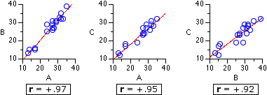
Figure 15.3 shows these intercorrelations for the k=3 example considered in the present chapter. As you can see, they do all come out positive and of approximately the same magnitude.

Figure 15.3. Intercorrelations among Groups A, B, and C

Note incidentally that the degree of intercorrelation among the k groups of measures is directly related to SSsubj, which is the aggregate measure of individual differences among the subjects in a repeated measures design, or among the matched sets of subjects in a randomized blocks design. The greater the degree of intercorrelation, the greater will be the size of SSsubj.

---

¶Post-ANOVA Comparisons: the Tukey HSD Test

In the independent-samples version of ANOVA, the "error term" of the F-ratio (the quantity that appears in the denominator) is MS_wg. In the correlated-samples version, it is MS_error. The Tukey HSD test introduced in Chapter 14, Part 2, can be extended to the correlated-samples version through the simple strategy of using MS_error in place of MS_wg and df_error in place of df_wg. Since the number of measures per group is equal to the number of subjects in a repeated measures design, or to the number of matched sets of subjects in a randomized blocks design, we will also be substituting N_subj for N_p/s.

For the example considered in the present chapter, recallTthat   MSerror=3.0,dferror=34,Nsubj=18,K=3

Here again is the calculator for critical values of Q for the .05 and .01 levels of significance. It is exactly the same calculator that appeared in Chapter 14, except now the entry for df is subscripted as df_error. Recall that values of K must fall between 3 and 10, inclusive.

---

Critical Values of Q

k	dfwg		Q.05	Q.01

---

Entering k=3 and df_error=34, the critical values come out as Q_.05=3.47 and Q_.01=4.42. Our calculations for HSD are therefore for the .05 level:

	HSD.05	=	Q.05 x sqrt	[	MSerror Nsubj	]		That is: In order to be considered significant at or beyond the .05 level, the difference between any two particular group means (larger—smaller) must be equal to or greater than 1.42.
		=	3.47 x sqrt	[	3.0 18	]
		=	1.42

and for the .01 level:

	HSD.01	=	Q.01 x sqrt	[	MSerror Nsubj	]		That is: In order to be considered significant at or beyond the .01 level, the difference between any two particular group means (larger—smaller) must be equal to or greater than 1.8.
		=	4.42 x sqrt	[	3.0 18	]
		=	1.8

The blue entries in the following table show the differences (larger—smaller) between each pair of group means in the example. As you can see, the comparisons for A·C and B·C are significant beyond the .01 level, while the one for A·B fails to achieve significance even at the basic .05 level.

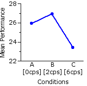
	A·B	Ma=25.9 Mb=26.9	1.0	HSD.05 = 1.42 HSD.01 = 1.8
	A·C	Ma=25.9 Mc=23.4	2.5
	B·C	Mb=26.9 Mc=23.4	3.5

Our investigator would therefore be able to conclude that performance on the rotary pursuit task is better under the 0cps and 2cps condition than it is under the 6cps condition. Notwithstanding the fact that M_b is greater than M_a, she would not be able to conclude that performance is better under the 2cps condition than under the 0cps condition.

---

¶Step-by-Step Computational Procedure: One-Way Analysis of Variance for Correlated Samples

Here again I will show the procedures for one particular value of k, namely k=3. The modifications required for different values will be fairly obvious. The steps listed below assume that you have already done the basic number-crunching to get X_i and X²_i for each of the k groups of measures and for all k groups combined. They also require the prior calculation of X_subj* for each subject in a repeated measures design, or for each set of matched subjects in a randomized blocks design.

---

Step 1. Combining all k groups of measures together, calculate

SST = ∑X2i —

(∑Xi)2 NT

---

Step 2. For each of the k groups separately, calculate the sum of squared deviates within the group ("g") as

SSg = ∑X2gi —

(∑Xgi)2 Ng

---

Step 3. Take the sum of the SS_g values across all k groups to get

SSwg = SSa+SSb+SSc

---

Step 4. Calculate SS_bg as

SSbg = SST—SSwg

---

Step 4a. Check your calculations up to this point by calculating SS_bg separately as

SSbg

=

(∑Xai)2 Na

+

(∑Xbi)2 Nb

+

(∑Xci)2 Nc

—

(∑XT)2 NT

---

Step 5. Calculate SS_subj as

SSsubj

=

(∑Xsubj*)2 k

—

(∑XTi)2 NT

---

Step 6. Calculate SS_error as

SSerror = SSwg — SSsubj

---

Step 7. Calculate the relevant degrees of freedom as

	dfT = NT—1dfbg = k—1dfwg = NT—k
	dfsubj = Nsubj—1dferror = dfwg—dfsubj

---

Step 8. Calculate the relevant mean-square values as

	MSbg	=	SSbg dfbg
and
	MSerror	=	SSerror dferror

---

Step 9. Calculate F as

F

=

MSbg MSerror

---

Step 10. Refer the calculated value of F to the table of critical values of F (Appendix D), with the appropriate pair of numerator/denominator degrees of freedom, as described earlier in this chapter.

---

---

Note that this chapter includes a subchapter on the Friedman Test, which is a non-parametric alternative to the one-way ANOVA for correlated samples.