©Richard Lowry, 1999-
All rights reserved.
Chapter 16.
Two-Way Analysis of Variance for Independent Samples
Part 1
As indicated in Chapter 13, the two-way ANOVA is a procedure that examines the effects of two independent variables concurrently. This not only provides a kind of economy in allowing you to look at two things for the price of one. It also, and often much more importantly, allows you to determine whether the two independent variables interact with respect to their effect on the dependent variable.
I will introduce this critically important concept with the familiar example of drug interactions. Suppose we were interested in the effects of two drugs, A and B, on the blood level of a certain hormone. To this end, we randomly and independently sort the members of our subject pool (healthy adult human males between the ages of 30 and 40) into four equal-sized groups. As shown in the following table, group r1c1("r"=row, "c"=column) serves as a kind of control group, receiving only an inert placebo containing zero units of A and zero units of B. Group r1c2 receives zero units of A and 1 unit of B; r2c1 receives 1 unit of A and zero units of B; and r2c2 receives 1 unit each of A and B.
The following tables and graphs show four possible scenarios. The numbers inside the blue cells in the table represent the respective mean blood levels of the hormone for each of the four groups following adminstration of the experimental treatment; the numbers to the right of each row and at the bottom of each column represent the mean for that particular row or column; and the number in the bottom right corner is the mean of the entire array. The adjacent graph in each scenario is a plot of the group mean values appearing in the blue cells.
Scenario 1|
One need not know much about statistical inference to surmise that the two drugs in this scenario show no effect at all, either separately or in combination. This is what would be expected on the basis of the null hypothesis.
Scenario 2|
In this scenario both drugs appear to increase the level of the hormone, but note that their combined effect is one of simple addition. With zero units of A and B, the mean blood level of the hormone is 5. Add 1 unit of B and it increases to 10. Start again from zero, add 1 unit of A, and it also increases from 5 to 10. When presented alone, 1 unit of either A or B increases the level of the hormone by 5. When presented together, they increase it by5+5 to 15. The effect of the two drugs in combination is merely the sum of the effects they have separately.
Scenario 3|
Here the drugs when presented separately are having the same effects as in Scenario 2, but now they are also interacting. The effect of the two when presented in combination is greater than the sum of their separate effects.
Scenario 4|
Here, too, is an interaction effect, but in the opposite direction. In Scenario 3 combining the drugs enhances their separate effects. Now the combined effect is one of mutual cancellation.
These are by no means the only sorts of interaction effects that can be found, though I think they will give you at least a preliminary idea of what the concept is pointing to. Whenever two variables in combination produce effects that are different from the simple sum of their separate effects, you have the makings of an interaction. When represented graphically, the absence of an interaction will appear as lines that are approximately parallel, as in Scenario 2, while the presence of an interaction will appear as lines that diverge or converge or cross over each other, as in Scenarios 3 and 4.
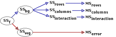
¶Procedure
Up to a point, the two-way ANOVA for independent samples proceeds exactly like the corresponding one-way ANOVA. Here as well, SSbg is the measure of the aggregate differences among the several groups, and SSwg is the measure of random variability inside the groups. The latter, SSwg, is treated the same way as in the one-way analysis: it ends up as the MSerror that appears in the denominator of theF-ratio. But now, with two independent variables and the data arrayed in the form of a rows-by-columns matrix, SSbg can be further divided, like Caesar's Gaul and Freud's psychical topography, into three parts. As illustrated in the following diagram, one of these parts measures the differences among the means of the two or more rows, another measures the mean differences among the two or more columns, and the third is a measure of the degree to which the two independent variables interact. Each of these three components is then converted into a corresponding value of MS, with the result that there are now three separate F-ratios to calculate and three separate tests of significance to perform: one for the row variable, one for the column variable, and one for the interaction between the two variables.
The two-way ANOVA is sufficiently important to warrant illustration with several examples. The first two are variations on the simple drug A versus drug B scenarios we have just examined. The third will be a bit more complex.
I will introduce this critically important concept with the familiar example of drug interactions. Suppose we were interested in the effects of two drugs, A and B, on the blood level of a certain hormone. To this end, we randomly and independently sort the members of our subject pool (healthy adult human males between the ages of 30 and 40) into four equal-sized groups. As shown in the following table, group r1c1
Note that the data structure in the two-variable case takes the form of a rows-by-columns matrix. For economy of expression, it is conventional to speak of the "row variable" and the "column variable" in accordance with how the two independent variables are arrayed in the matrix. In the present example, drug A is the row variable and drug B is the column variable. |
Drug B| 0 units | 1 unit | Drug | A 0 | units r1c1 | 0 units of A 0 units of B r1c2 | 0 units of A 1 unit of B 1 | unit r2c1 | 1 unit of A 0 units of B r2c2 | 1 unit of A 1 unit of B | |||
The following tables and graphs show four possible scenarios. The numbers inside the blue cells in the table represent the respective mean blood levels of the hormone for each of the four groups following adminstration of the experimental treatment; the numbers to the right of each row and at the bottom of each column represent the mean for that particular row or column; and the number in the bottom right corner is the mean of the entire array. The adjacent graph in each scenario is a plot of the group mean values appearing in the blue cells.
Scenario 1|
| Drug B | 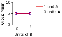
| ||||||||||||||
| 0 units | 1 unit | Drug | A 0 | units 5 | 5 | 5 | 1 | unit 5 | 5 | 5 |
| 5 | 5 | 5 | | |
One need not know much about statistical inference to surmise that the two drugs in this scenario show no effect at all, either separately or in combination. This is what would be expected on the basis of the null hypothesis.
Scenario 2|
| Drug B | 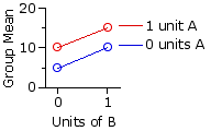
| ||||||||||||||
| 0 units | 1 unit | Drug | A 0 | units 5 | 10 | 7.5 | 1 | unit 10 | 15 | 12.5 |
| 7.5 | 12.5 | 10 | | |
In this scenario both drugs appear to increase the level of the hormone, but note that their combined effect is one of simple addition. With zero units of A and B, the mean blood level of the hormone is 5. Add 1 unit of B and it increases to 10. Start again from zero, add 1 unit of A, and it also increases from 5 to 10. When presented alone, 1 unit of either A or B increases the level of the hormone by 5. When presented together, they increase it by
In considering the effects of the two independent variables separately, what the two-way ANOVA actually looks at are the differences among the means of the row variable and the differences among the means of the column variable. By convention, these two sets of differences are spoken of as the "main effects" of the analysis, as distinguished from the "interaction effect," which is something above and beyond the two main effects. Thus, for the present scenario, the main effect for the row variable, drug A, is the difference between |
Scenario 3|
| Drug B | 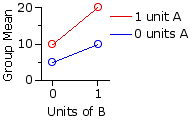
| ||||||||||||||
| 0 units | 1 unit | Drug | A 0 | units 5 | 10 | 7.5 | 1 | unit 10 | 20 | 15 |
| 7.5 | 15 | 11.25 | | |
Here the drugs when presented separately are having the same effects as in Scenario 2, but now they are also interacting. The effect of the two when presented in combination is greater than the sum of their separate effects.
Note again that the main effects would consist of the difference between |
Scenario 4|
| Drug B | 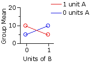
| ||||||||||||||
| 0 units | 1 unit | Drug | A 0 | units 5 | 10 | 7.5 | 1 | unit 10 | 5 | 7.5 |
| 7.5 | 7.5 | 7.5 | | |
Here, too, is an interaction effect, but in the opposite direction. In Scenario 3 combining the drugs enhances their separate effects. Now the combined effect is one of mutual cancellation.
But note that in this scenario there would be no main effects for either rows or columns |
These are by no means the only sorts of interaction effects that can be found, though I think they will give you at least a preliminary idea of what the concept is pointing to. Whenever two variables in combination produce effects that are different from the simple sum of their separate effects, you have the makings of an interaction. When represented graphically, the absence of an interaction will appear as lines that are approximately parallel, as in Scenario 2, while the presence of an interaction will appear as lines that diverge or converge or cross over each other, as in Scenarios 3 and 4.
¶Procedure
Up to a point, the two-way ANOVA for independent samples proceeds exactly like the corresponding one-way ANOVA. Here as well, SSbg is the measure of the aggregate differences among the several groups, and SSwg is the measure of random variability inside the groups. The latter, SSwg, is treated the same way as in the one-way analysis: it ends up as the MSerror that appears in the denominator of the
The two-way ANOVA is sufficiently important to warrant illustration with several examples. The first two are variations on the simple drug A versus drug B scenarios we have just examined. The third will be a bit more complex.
End of Chapter 16, Part 1.
Return to Top of Chapter 16, Part 1
Go to Chapter 16, Part 2
| Home | Click this link only if the present page does not appear in a frameset headed by the logo Concepts and Applications of Inferential Statistics |