©Richard Lowry, 1999-
All rights reserved.
Chapter 16.
Two-Way Analysis of Variance for Independent Samples
Part 2
| raw data | B| 0 units | 1 unit | A | 0 | units
20.4 17.4 | 20.0 18.4 24.5 21.0 19.7 22.3 17.3 23.3
20.5 26.3 | 26.6 19.8 25.4 28.2 22.6 23.7 22.5 22.6 1 | unit
22.4 19.1 | 22.4 25.4 26.2 25.1 28.8 21.8 26.3 25.2
34.1 21.9 | 32.6 28.5 29.0 25.8 29.0 27.1 25.7 24.4 | ||
Performing the requisite number-crunching on this array yields the summary values shown in the next table. The values pertaining to the four groups of measures in the original table of raw data are subscripted as g1, g2, g3, and g4; those pertaining to the rows are subscripted as r1 and r2; and those pertaining to the columns are subscripted as c1 and c2. The values deriving from the entire array of data (all groups combined) are as usual subscripted "T." It is worth a moment of your time to look back and forth between the table above and the one below to make sure you have a clear sense of where the summary values are coming from. (Click here if you would like a printable summary of these and other relevant tables of information as you work your way through this example.)
| summary data | B| 0 units | 1 unit |
| rows | A | 0 | units
Ng1=10 | ∑Xg1=204.3 ∑X2g1=4226.3
Ng2=10 | ∑Xg2=238.2 ∑X2g2=5741.4
Nr1=20 | ∑Xr1=442.5 1 | unit
Ng3=10 | ∑Xg3=242.7 ∑X2g3=5961.34
Ng4=10 | ∑Xg4=278.1 ∑X2g4=7855.3
Nr2=20 | ∑Xr2=520.8
| columns |
Nc1=20 | ∑Xc1=447.0
Nc2=20 | ∑Xc2=516.3
NT=40 | ∑XT=963.3 ∑X2T=23784.4 | ||||||||
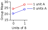
Up to this point it is all a tangle of numbers with no immediately discernible structure. It is only when you calculate the various means—for groups, rows, columns, and total array of data—that the pattern becomes visible. These means are given in the next table, along with a plot of the group means analogous to the ones shown in the earlier illustrations.
| means | B| 0 units | 1 unit |
| rows | 
A | 0 | units Mg1=20.43 |
Mg2=23.82 |
Mr1=22.13 | 1 | unit Mg3=24.27 | Mg4=27.81 | Mr2=26.04 |
| columns | Mc1=22.35 | Mc2=25.82 | MT=24.08 | | |||||||||
The resemblance between the above graph and the plot of our earlier Scenario 2 is no accident. When doing actual research, you must of course take your data as they come. The nice thing about generating illustrative data for a textbook is that you can shape them in any way you want. For this example I have deliberately arranged things so that there will be main effects for the row and column variables, but no interaction effect. The rationale is that understanding the presence of an interaction effect is best arrived at by first understanding its absence.
The next table shows the sums of squared deviates within each of the four groups, as well as for all four groups combined. These values are calculated exactly as they are in the corresponding one-way ANOVA, according to the general computational formula
| SS = ∑X2i — | (∑Xi)2 N |
| preliminary SS values | B| 0 units | 1 unit | A | 0 | units SSg1=52.44 |
SSg2=67.48 | 1 | unit SSg3=71.02 | SSg4=121.37 |
|
| SST=585.70 | | ||||
Also as in the one-way ANOVA, SSwg is given by the sum of the SS measures within the several groups. In the present case there are four groups; hence
| SSwg | = SSg1 + SSg2 + SSg3 + SSg4|
|
| = 52.44 + 67.48 + 71.02 + 121.37 |
|
| = 312.31 | |
The similarity continues for one more step, and then we shift gears. Once you have SST and SSwg, the measure of between-groups SS can be reached through simple subtraction:
| SSbg | = SST — SSwg|
|
| = 585.70 — 312.31 |
|
| = 273.39 | |
Here again I recommend performing a computational check by calculating SSbg from scratch. The structure is the same as before. The only difference is in the new subscriptions: g1, g2, etc. Please pay particularly close attention to this structure, for we will soon be applying it twice again with different casts of characters.
| SSbg | = | (∑Xg1)2 Ng1 | + | (∑Xg2)2 Ng2 | + | (∑Xg3)2 Ng3 | + | (∑Xg4)2 Ng4 | — | (∑XT)2 NT
|
|
| = | (204.3)2 | 10 + | (238.2)2 | 10 + | (242.7)2 | 10 + | (278.1)2 | 10 — | (963.3)2 | 40
|
|
| = | 273.39 | |
As indicated earlier, SSbg has three complementary components: one, SSrows, measures the differences among the means of the two or more rows; another, SScols, measures the mean differences among the two or more columns; and the third, SSinteraction, is a measure of the degree to which the row and column variables interact. To save space, we will henceforth refer to the interaction component as SSrxc, the subscription "rxc" being an abbreviation of the conventional shorthand expression "rows by columns."
For practical computational purposes, the simplest way to proceed is to calculate SSrows and SScols, and then subtract those two from SSbg to get the third component, SSrxc. Conceptually, the calculation of SSrows and SScols is exactly like the calculation of SSbg when you are doing it from scratch.
Consider the means of the two rows in our example:
| row 1 | row 2| observed row mean
| 22.13
| 26.04
| expected row mean
| 24.08
| 24.08
| deviate
| —1.95
| +1.96
| squared deviate
| 3.80
| 3.84
|
squared deviate weighted | by number in row (20) 76.0
| 76.8
| |
Take the sum of these two weighted squared deviates and you have
It is the same logic and procedure for SScols. The null hypothesis expects the means of the columns to be the same, and that can happen only if they are both equal
| col 1 | col 2| observed column mean
| 22.35
| 25.82
| expected column mean
| 24.08
| 24.08
| deviate
| —1.73
| +1.74
| squared deviate
| 2.99
| 3.03
|
squared deviate weighted | by number in column (20) 59.8
| 60.6
| |
Hence
I have marked both of the above values as "tentative" because calculations that start out with rounded numbers are at risk of accumulating substantial rounding errors. For practical purposes it is better to use the following computational formulas. Both follow the same basic pattern as when you are calculating SSbg from scratch
| SSbg | = | (∑Xg1)2 Ng1 | + | (∑Xg2)2 Ng2 | + | (∑Xg3)2 Ng3 | + | (∑Xg4)2 Ng4 | — | (∑XT)2 NT |
only now the items to the left of the minus sign pertain not to the individual groups of measures, but to the rows or the columns.
| SSrows | = | (∑Xr1)2 Nr1 | + | (∑Xr2)2 Nr2 | — | (∑XT)2 NT |
Click here if you would like a printable summary of the data on which these calculations are based.
|
|
| = | (442.5)2 | 20 + | (520.8)2 | 20 — | (963.3)2 | 40
|
|
| = | 153.27 | |
| SScols | = | (∑Xc1)2 Nc1 | + | (∑Xc2)2 Nc2 | — | (∑XT)2 NT
|
|
| = | (447.0)2 | 20 + | (516.3)2 | 20 — | (963.3)2 | 40
|
|
| = | 120.06 | |
Once you have these two components of SSbg, the SS measure of interaction can then be reached through simple subtraction:
| SSrxc | = SSbg — SSrows — SScols|
|
| = 273.39 — 153.27 — 120.06 |
|
| = 0.06 | |
As promised, the interaction effect in this example is essentially zero. The advantage of the simple subtractive procedure by which we have arrived at this conclusion is that it is quick and easy. The disadvantage is that does not give the slightest clue of the underlying logic of the process. The following procedure is more cumbersome and more prone to rounding errors, though at the same time more revealing of the inner workings of SSrxc.
It begins once again with the concept of the null hypothesis. To streamline things a bit, we will first lay out some items of symbolic notation:T
| Mg* = | the mean of any particular one of the the individual groups of measures
|
| Mr* =
| the mean of the row to which that group belongs
|
| Mc* =
| the mean of the column to which that group belongs
| |
If there is zero interaction between the row and column variables, then the mean of any particular one of the the individual groups, Mg*, should be a simple additive combination of Mr* and Mc*. The specific form of the combination is
| [null]Mg* = Mr* + Mc* — MT | Click here for a brief account of the logic of this formula. |
Thus, for group 1, which falls in row 1 and column 1:
| [null]Mg1 | = Mr1 + Mc1 — MT
|
|
| = 22.13 + 22.35 — 24.08
|
|
| = 20.40
| |
For group 2, which falls in row 1 and column 2:
| [null]Mg2 | = Mr1 + Mc2 — MT
|
|
| = 22.13 + 25.82 — 24.08
|
|
| = 23.87
| |
Here is the same table of means you saw earlier, except now I also include (in red) the results of the calculation of [null]Mg* for each of the four groups. The observed means of the groups (20.43,
| means | B| 0 units | 1 unit |
| rows | A | 0 | units 20.43 | 20.40 23.82 | 23.87
Mr1=22.13 | 1 | unit 24.27 | 24.31 27.81 | 27.78 Mr2=26.04 |
| columns | Mc1=22.35 | Mc2=25.82 | MT=24.08 | | ||||||||
As you can see, there is only the tiniest bit of difference between the observed group means and the means that would be expected if there were no rows-by-columns interaction.
Here again is that familiar conceptual structure by which you can convert the differences between observed and expected mean values into a meaningful measure of SS:
| g1 | g2 | g3 | g4| observed group mean
| 20.43
| 23.82
| 24.27
| 27.81
| expected group mean
| 20.40
| 23.87
| 24.31
| 27.78
| deviate
| +0.03
| —0.05
| —0.04
| +0.03
| squared deviate
| 0.0009
| 0.0025
| 0.0016
| 0.0009
|
squared deviate weighted | by number in group (10) 0.009
| 0.025
| 0.016
| 0.009
| |
The sum of these weighted squared deviates comes out to the same
For those whose memories, like mine, fall short of being photographic, here is a summary of the several SS values we have now calculated for this example:
| Total: | SST = 585.70
|
|
| within groups:
| SSwg = 312.31
|
|
| between groups:
| SSbg = 273.39
|
|
| rows:
| SSrows = 153.27
|
|
| columns:
| SScols = 120.06
|
|
| interaction:
| SSrxc = 0.06
| |
The following table lists the respective degrees of freedom that are associated with these values of SS. Note that dfrxc, the degrees of freedom for rows-by-columns interaction, is calculated in the same way as for a two-dimensional (rows-by-columns) chi-square test; namely,
| dfrxc = (r—1)(c—1) | r = number of rows c = number of columns |
All the other df structures are much as you would expect on the basis of previously examined versions of ANOVA. Note that the number of individual groups, or cells, in a rows-by-columns matrix is always equal to the product of r multiplied by c, rendered here as "rc." Thus, for the present example,
| in general | for the present example Total
| dfT = NT—1
| 40—1=39
| Note thatT | dfT=dfwg+dfbg within- | groups (error) dfwg = NT—rc
| 40—(2)(2)=36
| between- | groups dfbg = rc—1
| (2)(2)—1=3
| rows
| dfrows = r—1
| 2—1=1
| Note thatT | dfbg=dfrows+dfcols+dfrxc columns
| dfcols = c—1
| 2—1=1
| interaction
| dfrxc = (r—1)(c—1)
| (2—1)(2—1)=1
| |
As in previous versions of ANOVA, the relevant values of MS are in each case given by the ratio SS/df. Thus, for rows, columns, and interaction:
| MSrows | = | SSrows dfrows | MScols | = | SScols dfcols | MSrxc | = | SSrxc dfrxc
|
|
| = | 153.27 | 1
|
| = | 120.06 | 1
|
| = | 0.06 | 1
|
|
| = | 153.27 |
|
| = | 120.06 |
|
| = | 0.06 |
|
|
| | ||||||||||||
| MSerror | = | SSwg dfwg
|
|
| = | 312.31 | 36 = 8.68 | |
AndThere are the three bottom lines of the analysis:
| Frows | = | MSrows MSerror | Fcols | = | MScols MSerror | Frxc | = | MSrxc MSerror
|
|
| = | 153.27 | 8.68
|
| = | 120.06 | 8.68
|
| = | 0.06 | 8.68
|
|
| = | 17.67 |
|
| = | 13.84 |
|
| = | 0.01 |
| with df=1,36
| with df=1,36
| with df=1,36 | ||||||||||||
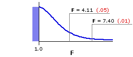
Figure 16.1 shows the sampling distribution of F for
Figure 16.1. Sampling Distribution of F for df=1,36

| |||||||||||||||
| df denomi- nator | df numerator| 1 | 2 | 3 | 36 | 4.11 | 7.40 3.26 | 5.25 2.87 | 4.38
| | ||||||
Clearly our miniscule value of
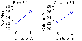
The fundamental meaning of the significant row and column effects is that the difference between the two row means

| col 1 [B=0] | col 2 [B=1] | row means row 1 | [A=0] |
| 22.13 | row 2 | [A=1] |
| 26.04 | column | means 22.35 | 25.82 | |
But for the present example it is all plain and simple. Each of the two drugs appears to increase arousal, and there is no indication that they interact with each other. When presented in combination, their effects are merely additive.
| Source | SS | df | MS | F | P| between groups | 273.39 | 1 | rows | 153.27 | 1 | 153.27 | 17.67 | <.01 | columns | 120.06 | 1 | 120.06 | 13.84 | <.01 | interaction | 0.06 | 1 | 0.06 | 0.01 | ns | within groups | (error) 312.31 | 36 | 8.68 | TOTAL | 585.70 | 39 | "ns" = "non-significant" | | ||||||
End of Chapter 16, Part 2.
Return to Top of Chapter 16, Part 2
Go to Chapter 16, Part 3
| Home | Click this link only if the present page does not appear in a frameset headed by the logo Concepts and Applications of Inferential Statistics |