Our second example uses the same research setting as in Example 1 and, as you will see in a moment, almost the same data. Now that we have laid the groundwork for the two-way independent-samples ANOVA, the computational side of this example will be quick and easy. The tricky part will the interpretation of the results, once we have them.

First a reminder of the setting: To test the separate and mutual effects of two drugs, A and B, on physiological arousal, researchers randomly and independently sorted 40 laboratory rats into four groups of 10 subjects each. Each group received a certain dosage of drug A (zero units or 1 unit) and a certain dosage of drug B (zero units or 1 unit). The dependent variable was a standard measure of physiological arousal. One of the groups served as a control, receiving only an inert placebo containing zero units of A and zero units of B.

The following table shows the consequent measures of physiological arousal for each subject in each of the four groups. If you have a sharp eye and a keen memory, you will see that all of the values listed for groups 1, 2, and 3 are the same as in Example 1. The only difference is in the listing for group 4, whose members receive 1 unit of A and 1 unit of B.

raw data		B
		0 units	1 unit
A	0 units	20.4 17.4   20.0 18.4   24.5 21.0   19.7 22.3   17.3 23.3	20.5 26.3   26.6 19.8   25.4 28.2   22.6 23.7   22.5 22.6
	1 unit	22.4 19.1   22.4 25.4   26.2 25.1   28.8 21.8   26.3 25.2	17.5 13.6   16.9 12.4   16.4 18.3   13.6 19.1   16.1 20.5

As the procedure follows the same format we worked through in Example 1, we will zip through it with only a minimum of commentary. (Click here if you would like a printable summary of the raw data and summary values for this example.)

---

Summary Values from Preliminary Number-Crunching

summary data		B
		0 units	1 unit		rows
A	0 units	Ng1=10 ∑Xg1=204.3 ∑X2g1=4226.3	Ng2=10 ∑Xg2=238.2 ∑X2g2=5741.4		Nr1=20 ∑Xr1=442.5
	1 unit	Ng3=10 ∑Xg3=242.7 ∑X2g3=5961.35	Ng4=10 ∑Xg4=164.4 ∑X2g4=2763.66		Nr2=20 ∑Xr2=407.1
	columns	Nc1=20 ∑Xc1=447.0	Nc2=20 ∑Xc2=402.6	NT=40 ∑XT=849.6 ∑X2T=18692.7

---

Means and Graph of Group Means

		B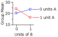
		0 units	1 unit		rows
A	0 units	Mg1=20.43	Mg2=23.82		Mr1=22.13
	1 unit	Mg3=24.27	Mg4=16.44		Mr2=20.36
	columns	Mc1=22.35	Mc2=20.13	MT=21.24

---

Preliminary SS Values

		B
		0 units	1 unit
A	0 units	SSg1=52.45	SSg2=67.48
	1 unit	SSg3=71.02	SSg4=60.92
				SST=647.2

---

	SSwg	= SSg1 + SSg2 + SSg3 + SSg4
		= 52.45 + 67.48 + 71.02 + 60.92
		= 251.87

---

	SSbg	= SST — SSwg
		= 647.2 — 251.87
		= 395.33

---

	SSrows	=	(∑Xr1)2 Nr1	+	(∑Xr2)2 Nr2	—	(∑XT)2 NT
		=	(442.5)2 20	+	(407.1)2 20	—	(849.6)2 40
		=	31.33

---

	SScols	=	(∑Xc1)2 Nc1	+	(∑Xc2)2 Nc2	—	(∑XT)2 NT
		=	(447.0)2 20	+	(402.6)2 20	—	(849.6)2 40
		=	49.28

---

	SSrxc	= SSbg — SSrows — SScols
		= 395.33 — 31.33 — 49.28
		= 314.72

---

The following table shows (in red) the values of [null]M_g* for each of the four groups, as calculated by the method described in connection with Example 1. As before, the observed means of the groups (20.43, 23.82, etc.) appear in black. The graphs below the table show the observed group means in comparison with the pattern that would be expected if there were zero interaction between the row and column variables. As you can see from both the table and the graphs, there is a substantial difference between the observed and the expected.

means		B
		0 units	1 unit		rows
A	0 units	20.43 23.24	23.82 21.02		Mr1=22.13
	1 unit	24.27 21.47	16.44 19.25		Mr2=20.36
	columns	Mc1=22.35	Mc2=20.13	MT=21.24

observed

expected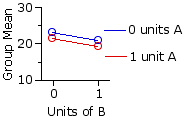

---

Degrees of Freedom

degrees of freedom	in general	for the present example
Total	dfT = NT—1	40—1=39
within-  groups  (error)	dfwg = NT—rc	40—(2)(2)=36
between-  groups	dfbg = rc—1	(2)(2)—1=3
rows	dfrows = r—1	2—1=1
columns	dfcols = c—1	2—1=1
interaction	dfrxc = (r—1)(c—1)	(2—1)(2—1)=1

---

MS Values

	MSrows	=	SSrows dfrows		MScols	=	SScols dfcols		MSrxc	=	SSrxc dfrxc
		=	31.33 1			=	49.28 1			=	314.72 1
		=	31.33			=	49.28			=	314.72

	MSerror	=	SSwg dfwg
		=	251.87 36	= 7.0

---

F-ratios

	Frows	=	MSrows MSerror		Fcols	=	MScols MSerror		Frxc	=	MSrxc MSerror
		=	31.33 7.0			=	49.28 7.0			=	314.72 7.0
		=	4.48			=	7.04			=	44.94
	with df=1,36				with df=1,36				with df=1,36

---

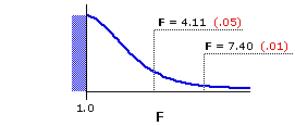
Here again is the sampling distribution of F for df=1,36, along with the corresponding tabular portion of Appendix D. The critical values for the .05 and .01 levels of significance are F=4.11 and F=7.40, respectively.

Figure 16.2. Sampling Distribution of F for df=1,36

	df denomi- nator	df numerator
		1	2	3
	36	4.11 7.40	3.26 5.25	2.87 4.38

In brief, all three of the effects are significant: the main effects for rows and columns (F_rows=4.47, F_cols=7.03) both beyond the .05 level, and the large interaction effect (F_rxc=44.88) far beyond the .01 level. This is the easy part of the analysis. Now for the trickier part, which is to figure out what it means.

---

Once again, the fundamental meaning of the significant row and column effects is that the difference between the two row means (22.13 vs 20.36) and the difference between the two column means (22.35 vs 20.13) each reflect something more than mere random variability. But note what happens when you simply take these two differences at face value, without reference to the very substantial interaction effect. As indicated by the following plots of the row and column means, the "obvious" inference is that drugs A and B both decrease arousal.

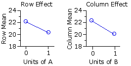
Examine the data in closer detail, however, and you will see that this conclusion is quite the opposite of what is really happening. For group 1, which receives only the inert placebo, the mean level of arousal is 20.43. For group 2, which receives 1 unit of B and none of A, it is higher: 23.82. For group 3, which receives 1 unit of A and none of B, it is also higher: 24.27. The complication comes with group 4, which receives 1 unit each of A and B; for here the effects of the two drugs in combination are not merely additive.

		B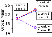
		0 units	1 unit
A	0 units	Mg1=20.43	Mg2=23.82
	1 unit	Mg3=24.27	Mg4=16.44

Indeed, they are the very opposite of additive: A and B in combination produce a mean arousal level of 16.44, substantially lower than the 20.43 observed with the inert placebo group. Presented separately, each of the two drugs increases arousal, while in combination they interact to produce a marked decrease in arousal.

Although the above graph captures the texture of the interaction effect in this particular example, the more generic format is the one shown earlier (now adjacent), in which the individual group means are plotted across their respective rows. The fundamental generic meaning of a significant interaction effect is that the difference between			Interaction Effect
	(i)	the observed pattern of group means and
	(ii)	the pattern that would be expected if the combined effects of the row and column variables were merely additive
reflects something more than mere random variability.

---

ANOVA Summary Table

	Source	SS	df	MS	F	P
	between groups	395.19	3
	rows	31.33	1	31.33	4.48	<.05
	columns	49.28	1	49.28	7.04	<.05
	interaction	314.72	1	314.72	44.96	<.01
	within groups (error)	251.87	36	7.0
	TOTAL	647.2	39

---