©Richard Lowry, 1999-
All rights reserved.
Subchapter 15a.
The Friedman Test for 3 or More Correlated Samples
Assumptions of one-way ANOVA for correlated samples (see text of Chapter 15 for details)
~equal-interval scale of measurement
~independence of measures within each group
~normal distribution of source population(s)
~equal variances among groups
~homogeneity of covariance
~equal-interval scale of measurement
~independence of measures within each group
~normal distribution of source population(s)
~equal variances among groups
~homogeneity of covariance
We have noted several times that the analysis of variance is quite robust with respect to the violation of its assumptions, providing that the k groups are all of the same size. In the correlated-samples ANOVA this provision is always satisfied, since the number of measures in each of the groups is necessarily equal to the number of subjects in the repeated-measures design, or to the number of matched sets in the randomized blocks design.
Still, there are are certain kinds of correlated-samples situations where the violation of one or more assumptions might be so thorough-going as to cast doubt on any result produced by an analysis of variance. In cases of this sort, a useful non-parametric alternative can be found in a rank-based procedure known as the Friedman Test.
And the|second would be the case where these measures start out as mere ratings.|
In both of these situations the assumption of an equal-interval scale of measurement is clearly not met. There's a good chance that the assumption of a normal distribution of the source population(s) would also not be met. Other cases where the equal-interval assumption will be thoroughly violated include those in which the scale of measurement is intrinsically non-linear: for example, the decibel scale of sound intensity, the Richter scale of earthquake intensity, or any logarithmic scale.
I will illustrate the Friedman test with a rating-scale example that is close to my amateur violinist's heart. The venerable auction house of Snootly & Snobs will soon be putting three fine 17th-and 18th-century violins, A, B, and C, up for bidding. A certain musical arts foundation, wishing to determine which of these instruments to add to its collection, arranges to have them played by each of 10 concert violinists. The players are blindfolded, so that they cannot tell which violin is which; and each plays the violins in a randomly determined sequence (BCA, ACB, etc.).
They are not informed that the instruments are classic masterworks; all they know is that they are playing three different violins. After each violin is played, the player rates the instrument on a 10-point scale of overall excellence(1=lowest, 10=highest). The players are told that they can also give fractional ratings, such as 6.2 or 4.5, if they wish. The results are shown in the adjacent table. For the sake of consistency, the n=10 players are listed as "subjects."
¶Logic and Procedure
The Friedman test begins by rank-ordering the measures for each subject. For the present example we will assign the rank of "3" to the largest of a subject's three measures, "2" to the intermediate of the three, and "1" to the smallest. Thus for subject 1, the largest measure is in column A, the next largest in column B, and the smallest in column C; so the sequence of ranks across the row for subject 1 is 3,2,1. For subject 2 it is 3,1,2. And so forth. (The guidelines for assigning tied ranks are described in Subchapter 11a in connection with the Mann-Whitney test.)
The null hypothesis in this scenario is that the three violins do not differ with respect to whatever it is that blindfolded expert players would judge to be the overall excellence of an instrument.
This would entail that each of the six possible sequences of A,B,C ranks
1,2,3
1,3,2
2,1,3
2,3,1
3,1,2
3,2,1
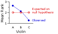
is equally likely, hence that the three columns will tend to include a random jumble of 1's, 2's, and 3's, in approximately equal proportions. In this case, the sums and the means of the columns would also tend to come out approximately the same.
 In most respects you will find the logic of the Friedman test quite similar to that of the Kruskal-Wallis test examined in Subchapter 14a. For any particular value of k (the number of measures per subject), the mean of the ranks for any particular one of the n subjects is
 (k+1)/2.
Thus for k=3, as in the present example, it is4/2=2; for k=4, it would be 5/2=2.5; and so on. On the null hypothesis, this would also be the expected value of the mean for each of the k columns. Similarly, the expected value for each of the column sums would be this amount multiplied by the number of subjects: n(k+1)/2. For the present example, with n=10, it would be (10)(4)/2=20.
The following items of symbolic notation are the same ones we used in connection with the Kruskal-Wallis test:
·The Measure of Aggregate Group Differences
Also the same as in the Kruskal-Wallis test is the measure of the aggregate degree to which the k group means differ. It is the between-groups sum of squared deviates defined in Subchapter 14a as SSbg(R), the "(R)" serving as a reminder that this particular version of SSbg is based on ranks. The following table summarizes the values needed for the calculation of SSbg(R).
As in all other cases heretofore examined, the squared deviate for any particular group mean is equal to the squared difference between that group mean and the mean of the overall array of data, multiplied by the number of observations on which the group mean is based. Thus, for each of our current three groups
Except now, since each group is necessarily of the same size, it can be reduced to the simpler form
For the same reason, the computational formula (less susceptible to rounding errors) can take the simpler form
For the present example, with n=10, k=3, and values of Tg and Tall as indicated above, this would come out as
·The Sampling Distribution of SSbg(R)
When we examined the Kruskal-Wallis test in Subchapter 14a, we saw that SSbg(R) can be converted into the measure designated as H, which can then be referred to the sampling distribution of chi-square fordf=k—1. The same is true of the Friedman test; the only difference is in the details of the conversion. For the Friedman test, the resulting measure is spoken of simply as a value of chi-square and takes the form
which for the present example comes out as
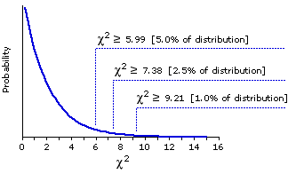
The following graph is borrowed once again from Chapter 8. As you can see, the observed valueof  =9.95,
 when referred to the appropriate sampling distribution of chi-square, is significant beyond the .01 level.
 Our musical arts foundation can therefore conclude with considerable confidence that the observed differences among the mean rankings for the three violins reflect something more than mere random variability, something more than mere chance coincidence among the judgments of the expert players.
·An Alternative Computational Formula
Textbook accounts of the Friedman test usually give a different computational formula for chi-square. Its advantage is that it can be (slightly) more convenient to use. Its disadvantage is that it does not give you the faintest idea of just what the measure is measuring. But here it is anyway, just in case you ever need to recognize it.
As you can see in connection with our present example, the result comes out quite the same either way.
Still, there are are certain kinds of correlated-samples situations where the violation of one or more assumptions might be so thorough-going as to cast doubt on any result produced by an analysis of variance. In cases of this sort, a useful non-parametric alternative can be found in a rank-based procedure known as the Friedman Test.
There are two kinds of correlated-samples situations where the advisability of the non-parametric alternative would be fairly obvious. The first would be the case where the k measures for each subject start out as mere rank-orderings.|
|
E.g.: To assess the likely results of an upcomming election, the 30 members of a presumably representative "focus group" of eligible voters are each asked to rank the 3 candidates, A, B, and C, in the order of their preference (1=most preferred, 3=least preferred). |
|
E.g.: The members of the "focus group" are instead asked to rate candidates on a 10-point scale (1=lowest rating, 10=highest). |
In both of these situations the assumption of an equal-interval scale of measurement is clearly not met. There's a good chance that the assumption of a normal distribution of the source population(s) would also not be met. Other cases where the equal-interval assumption will be thoroughly violated include those in which the scale of measurement is intrinsically non-linear: for example, the decibel scale of sound intensity, the Richter scale of earthquake intensity, or any logarithmic scale.
Violin| subjects | A | B | C |
1 | 2 3 4 5 6 7 8 9 10
9.0 | 9.5 5.0 7.5 9.5 7.5 8.0 7.0 8.5 6.0
7.0 | 6.5 7.0 7.5 5.0 8.0 6.0 6.5 7.0 7.0
6.0 | 8.0 4.0 6.0 7.0 6.5 6.0 4.0 6.5 3.0 | |||
They are not informed that the instruments are classic masterworks; all they know is that they are playing three different violins. After each violin is played, the player rates the instrument on a 10-point scale of overall excellence
¶Logic and Procedure
| Original Measures | Ranked Measures| subjects | A | B | C | A | B | C |
1 | 2 3 4 5 6 7 8 9 10
9.0 | 9.5 5.0 7.5 9.5 7.5 8.0 7.0 8.5 6.0
7.0 | 6.5 7.0 7.5 5.0 8.0 6.0 6.5 7.0 7.0
6.0 | 8.0 4.0 6.0 7.0 6.5 6.0 4.0 6.5 3.0
3 | 3 2 2.5 3 2 3 3 3 2
2 | 1 3 2.5 1 3 1.5 2 2 3
1 | 2 1 1 2 1 1.5 1 1 1 | ||||||
Ranked Measures| subjects | A | B | C |
1 | 2 3 4 5 6 7 8 9 10
3 | 3 2 2.5 3 2 3 3 3 2
2 | 1 3 2.5 1 3 1.5 2 2 3
1 | 2 1 1 2 1 1.5 1 1 1 sums | 26.5 | 21.0 | 12.5 | means | 2.65 | 2.10 | 1.25 | | |||
This would entail that each of the six possible sequences of A,B,C ranks
1,2,3
1,3,2
2,1,3
2,3,1
3,1,2
3,2,1
is equally likely, hence that the three columns will tend to include a random jumble of 1's, 2's, and 3's, in approximately equal proportions. In this case, the sums and the means of the columns would also tend to come out approximately the same.

Thus for k=3, as in the present example, it is
The following items of symbolic notation are the same ones we used in connection with the Kruskal-Wallis test:
| TA = | the sum of the n ranks in column A|
| MA = | the mean of the n ranks in column A |
| TB = | the sum of the n ranks in column B |
| MB = | the mean of the n ranks in column B |
| TC = | the sum of the n ranks in column C |
| MC = | the mean of the n ranks in column C |
| Tall = | the sum of the nk ranks in all columns combined | [In all cases equal to nk(k+1)/2]T
| Mall = | the mean of the nk ranks in all columns combined | [In all cases equal to (k+1)/2] | |||||||||||||
·The Measure of Aggregate Group Differences
Also the same as in the Kruskal-Wallis test is the measure of the aggregate degree to which the k group means differ. It is the between-groups sum of squared deviates defined in Subchapter 14a as SSbg(R), the "(R)" serving as a reminder that this particular version of SSbg is based on ranks. The following table summarizes the values needed for the calculation of SSbg(R).
| A | B | C | All| counts | 10 | 10 | 10 | 30 |
n=10 [subjects]T | k=3 [measures per subject]T nk=30 sums | 26.5 | 21.0 | 12.5 | 60.0 | means | 2.65 | 2.10 | 1.25 | 2.0 | |
As in all other cases heretofore examined, the squared deviate for any particular group mean is equal to the squared difference between that group mean and the mean of the overall array of data, multiplied by the number of observations on which the group mean is based. Thus, for each of our current three groups
| A: | 10(2.65—2.0)2 = 4.225 | |||||||
| B: | 10(2.10—2.0)2 = 0.100
|
| C:
| 10(1.25—2.0)2 = 5.625
|
|
| SSbg(R) = 9.950 |
Once again we can write the conceptual formula for SSbg(R) as
| SSbg(R) =( | As usual, the subscript "g" means "any particular group." |
Except now, since each group is necessarily of the same size, it can be reduced to the simpler form
| SSbg(R) =(n | n = number of subjects |
For the same reason, the computational formula (less susceptible to rounding errors) can take the simpler form
| SSbg(R) | = | . na | — | (Tall)2 nka | n = number of subjectsT k = measures per subject |
For the present example, with n=10, k=3, and values of Tg and Tall as indicated above, this would come out as
| SSbg(R) | = | (26.5)2+(21.0)2+(12.5)2 10 | — | (60)2 30
|
|
| = | 9.95
| |
·The Sampling Distribution of SSbg(R)
When we examined the Kruskal-Wallis test in Subchapter 14a, we saw that SSbg(R) can be converted into the measure designated as H, which can then be referred to the sampling distribution of chi-square for
| x | = | SSbg(R) k(k+1)/12
| |
which for the present example comes out as
| x | = | 9.95 3(3+1)/12 | = | 9.95 1 | = 9.95|
| |
When k is equal to 3, the application of this "conversion" formula is merely pro forma; for in this case the denominator of the ratio will always come down to 3(4)/12=1, so the resulting value of chi-square will always be equal to SSbg(R). This, however, will not be so when k is something other than 3. With k=4 the denominator will be 4(5)/12=1.67; with k=5 it will be 5(6)/12=2.5; and so on.
The following graph is borrowed once again from Chapter 8. As you can see, the observed value
Theoretical Sampling Distribution of Chi-Square for df=2

|

·An Alternative Computational Formula
Textbook accounts of the Friedman test usually give a different computational formula for chi-square. Its advantage is that it can be (slightly) more convenient to use. Its disadvantage is that it does not give you the faintest idea of just what the measure is measuring. But here it is anyway, just in case you ever need to recognize it.
| x | = | 12 nk(k+1) | .|
| |
As you can see in connection with our present example, the result comes out quite the same either way.
| x | = | 12 (10)(3)(4) | [(26.5)2+(21.0)2+(12.5)2]x — (3)(10)(4)|
|
| = | (0.1 x 1299.5) — 120 = 9.95 |
| | |||
The VassarStats web site has a page that will perform all steps of the Friedman test, including the rank-ordering of the raw measures.
End of Subchapter 15a.
Return to Top of Subchapter 15a
Go to Chapter 16 [Two-Way Analysis of Variance for Independent Samples]
| Home | Click this link only if the present page does not appear in a frameset headed by the logo Concepts and Applications of Inferential Statistics |