©Richard Lowry, 1999-
All rights reserved.
Chapter 15.
One-Way Analysis of Variance for Correlated Samples
Part 1
You can think of this version of the analysis of variance as an extension of the correlated-samples t-test described in Chapter 12. The most conspicuous similarity between the two is in the way the data are arrayed. In the correlated-samples t-test we typically have a certain number of subjects, each measured under two conditions, A and B. Or alternatively, we have a certain number of matched pairs of subjects, with one member of the pair measured under condition A and the other measured under condition B.
It is the same structure with the correlated-samples ANOVA, except that now the number of conditions is three or more: A|B|C, A|B|C|D, and so forth. When the analysis involves each subject being measured under each of the k conditions, it is sometimes spoken of as a repeated measures or within subjects design. When it involves subjects matched in sets of three fork=3, four for k=4, and so on, with the subjects in each matched set randomly assigned to one or another of the k conditions, it is described as a randomized blocks design. (In this latter case, each set of k matched subjects constitutes a "block.") Thus, for k=3:
Repeated Measures|
Randomized Blocks|
In both versions, repeated measures and randomized blocks, the utility of the correlated-samples ANOVA is the same as for the correlated-samplest-test: it is highly effective in removing the extraneous variability that derives from pre-existing individual differences. It is the same point made in Chapter 12. In some cases individual differences might be the very essence of the phenomena that are of interest. But there are also many situations where they are merely irrelevant clutter.
Up to a point, the logic and procedure of the correlated-samples ANOVA are the same as for the independent-samples version described in Chapters 13 and 14. In the independent-samples ANOVA, SST is analyzed into two complementary components, SSbg and SSwg. Each of the latter, divided by its respective value of df, then yields a value of MS; and these, in turn, yield the F-ratio. The numerator of the ratio, MSbg, reflects the aggregate differences among the means of the k groups of measures; and the denominator, MSwg, reflects the random variability, commonly described as "error," that exists inside the k groups.
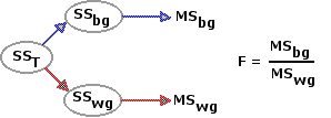
In most real-life situations, a certain amount of the variability that exists inside the k groups will reflect pre-existing individual differences among the subjects. In the medication experiment described in Chapter 14, for example, it is possible that the prior aversive conditioning had been more effective in some subjects than in others; or that some subjects were more prone to agitation than others; or simply that some were stronger than others and could therefore pull harder. Each of these sources of variability would be entirely extraneous to the question the investigators were aiming to answer. Of course, one way to avoid the extraneous clutter would be to ensure at the outset that all subjects are equally well conditioned, equally prone to agitation, equally strong, and so forth. But that would surely be more easily said than done.
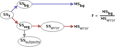
In the correlated-samples ANOVA, the extraneous clutter is not avoided. It is faced head-on, identified, and removed. Whether by repeated measures or randomized blocks, the correlated-samples design allows us to identify the portion of SSwg that is attributable to pre-existing individual differences. This portion, designated as SSsubjects, is dropped from the analysis; and the portion that remains, SSerror, is then used as the measure of sheer, cussed random variability.
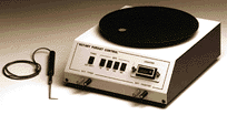
To illustrate the procedures we will take an another example involving sensory-motor coordination. The following picture and diagram represent a device known as a rotary pursuit apparatus, often used in psychological research as an instrument for measuring sensory-motor coordination. On its top is a turntable that can be set to rotate at pre-selected speeds. Toward the edge of the turntable is a metal disk (a) that revolves around the center of the turntable as the latter rotates. Connected to the apparatus is a hand-held stylus (B) with a metal tip. The subject's task is to pursue the revolving disk with the stylus, keeping the stylus in contact with the disk as much as possible. When the two are in contact an electrical circuit is closed, thus providing a record of how well the subject does on the task.
An investigator is interested in assessing the effects of rhythmic auditory stimulation on performance of the rotary pursuit task. To this end, she has each of 18 randomly selected human subjects perform the task under each of three conditions. In all conditions, the turntable rotates counter-clockwise at a constant rate of one rotation per second. In condition A there is no auditory stimulation other than the sound normally made by the apparatus. In the other two conditions the subject hears a periodic clicking sound. In condition B, the click occurs twice per second; and in condition C, six times per second. (The investigator selects these particular frequencies on certain theoretical grounds, which we need not go into.) To obviate the possibility of sequence effects, three of the subjects perform the task in the sequence ABC; three perform it in the sequence ACB; and so on for all the other of the six possible sequences: BAC, BCA, CAB, and CBA.
The following table shows the measures of how well each of the 18 subjects performed under each of thek=3 conditions. Also shown are the means of the three groups of measures and the mean performance of each individual subject across the three conditions. To emphasize the substantial individual differences that occur among the subjects, they are listed in the order of their respective individual mean levels of performance, from highest to lowest. Immediately below the table is Figure 15.1, showing the pattern of group means, A|B|C, in graphic form.
Figure 15.1. Mean Performance in Conditions A, B, and C
So here we are again: on the one hand, ostensible differences among the group means; and on the other, the ever-present possibility that the observed "effect" results from nothing more than mere random variability.
¶Parallels with the independent-samples ANOVA
The first few steps in the analysis are exactly the same as you saw in Chapter 14. Basic preliminary number-crunching on the data in columns A, B, and C of the above table yields the following values of∑Xi and ∑X2i for the three groups and for total array of data.
These in turn allow for the calculation of the following sums of squared deviates.
As in the independent-samples ANOVA, the within-groups SS is the sum of the k separate values of SSg (recall that the subscript "g" means "any particular group"). Thus
Similarly, the between-groups SS can then be calculated as
(SSbg) among the means of the 3 groups are rather tiny in comparison with the variability (SSwg) that occurs inside the groups. If you were performing the analysis as an independent-samples ANOVA, this would not be great news unless you were hoping to find a non-significant result. For that huge value of SSwg would also give you a large value of MSwg, hence a rather puny value of F.
As already mentioned, the virtue of the correlated-samples procedure is that it takes the analysis a step further. It has arranged things in advance so that it can identify the portion of SSwg that derives from pre-existing individual differences. And once identified, this portion—in the present case, a very large portion—can be removed. The details of identification and removal will be described in Part 2.
It is the same structure with the correlated-samples ANOVA, except that now the number of conditions is three or more: A|B|C, A|B|C|D, and so forth. When the analysis involves each subject being measured under each of the k conditions, it is sometimes spoken of as a repeated measures or within subjects design. When it involves subjects matched in sets of three for
Repeated Measures|
| Subject | A | B | C| 1 |
subj1 under | condition A
subj1 under | condition B
subj1 under | condition C Each row represents one subject measured under each of k conditions. 2 |
subj2 under | condition A
subj2 under | condition B
subj2 under | condition C 3 |
subj3 under | condition A
subj3 under | condition B
subj3 under | condition C And so on. | | ||||
Randomized Blocks|
| Block | A | B | C| 1 |
subj1a under | condition A
subj1b under | condition B
subj1c under | condition C Each row includes k matched subjects, each measured under one or another of the k conditions 2 |
subj2a under | condition A
subj2b under | condition B
subj2c under | condition C 3 |
subj3a under | condition A
subj3b under | condition B
subj3c under | condition C And so on. | | ||||
In both versions, repeated measures and randomized blocks, the utility of the correlated-samples ANOVA is the same as for the correlated-samples
Up to a point, the logic and procedure of the correlated-samples ANOVA are the same as for the independent-samples version described in Chapters 13 and 14. In the independent-samples ANOVA, SST is analyzed into two complementary components, SSbg and SSwg. Each of the latter, divided by its respective value of df, then yields a value of MS; and these, in turn, yield the F-ratio. The numerator of the ratio, MSbg, reflects the aggregate differences among the means of the k groups of measures; and the denominator, MSwg, reflects the random variability, commonly described as "error," that exists inside the k groups.

In most real-life situations, a certain amount of the variability that exists inside the k groups will reflect pre-existing individual differences among the subjects. In the medication experiment described in Chapter 14, for example, it is possible that the prior aversive conditioning had been more effective in some subjects than in others; or that some subjects were more prone to agitation than others; or simply that some were stronger than others and could therefore pull harder. Each of these sources of variability would be entirely extraneous to the question the investigators were aiming to answer. Of course, one way to avoid the extraneous clutter would be to ensure at the outset that all subjects are equally well conditioned, equally prone to agitation, equally strong, and so forth. But that would surely be more easily said than done.
In the correlated-samples ANOVA, the extraneous clutter is not avoided. It is faced head-on, identified, and removed. Whether by repeated measures or randomized blocks, the correlated-samples design allows us to identify the portion of SSwg that is attributable to pre-existing individual differences. This portion, designated as SSsubjects, is dropped from the analysis; and the portion that remains, SSerror, is then used as the measure of sheer, cussed random variability.

To illustrate the procedures we will take an another example involving sensory-motor coordination. The following picture and diagram represent a device known as a rotary pursuit apparatus, often used in psychological research as an instrument for measuring sensory-motor coordination. On its top is a turntable that can be set to rotate at pre-selected speeds. Toward the edge of the turntable is a metal disk (a) that revolves around the center of the turntable as the latter rotates. Connected to the apparatus is a hand-held stylus (B) with a metal tip. The subject's task is to pursue the revolving disk with the stylus, keeping the stylus in contact with the disk as much as possible. When the two are in contact an electrical circuit is closed, thus providing a record of how well the subject does on the task.
 Courtesy of Lafayette Instruments | 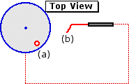
|
An investigator is interested in assessing the effects of rhythmic auditory stimulation on performance of the rotary pursuit task. To this end, she has each of 18 randomly selected human subjects perform the task under each of three conditions. In all conditions, the turntable rotates counter-clockwise at a constant rate of one rotation per second. In condition A there is no auditory stimulation other than the sound normally made by the apparatus. In the other two conditions the subject hears a periodic clicking sound. In condition B, the click occurs twice per second; and in condition C, six times per second. (The investigator selects these particular frequencies on certain theoretical grounds, which we need not go into.) To obviate the possibility of sequence effects, three of the subjects perform the task in the sequence ABC; three perform it in the sequence ACB; and so on for all the other of the six possible sequences: BAC, BCA, CAB, and CBA.
The following table shows the measures of how well each of the 18 subjects performed under each of the
| Conditions ("cps"=clicks per second) Sub- | jects A | [0cps] B | [2cps] C | [6cps]
| Subject | Means 1 | 2 3 4 5 6 7 8 9 10 11 12 13 14 15 16 17 18
35 | 32 33 32 31 29 29 27 27 28 27 27 24 24 17 17 14 13
39 | 35 32 32 33 30 31 29 31 27 27 26 29 25 16 15 15 13
32 | 31 28 29 26 29 27 27 24 24 23 23 19 19 18 17 12 13
35.3 | 32.7 31.0 31.0 30.0 29.3 29.0 27.7 27.3 26.3 25.7 25.3 24.0 22.7 17.0 16.3 13.7 13.0 Group | Means 25.9 | 26.9 | 23.4 | | |||
Figure 15.1. Mean Performance in Conditions A, B, and C
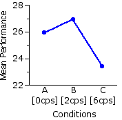
| Please keep in mind that the data in this example are completely imaginary. I do not know whether an actual experiment of this sort would produce a pattern of group means resembling the one shown here. |
So here we are again: on the one hand, ostensible differences among the group means; and on the other, the ever-present possibility that the observed "effect" results from nothing more than mere random variability.
¶Parallels with the independent-samples ANOVA
The first few steps in the analysis are exactly the same as you saw in Chapter 14. Basic preliminary number-crunching on the data in columns A, B, and C of the above table yields the following values of
| A [0cps] | B [2cps] | C [6cps] | All groups combined
| Na=18 | ∑Xai=466 ∑X2ai= 12800 Nb=18 | ∑Xbi=485 ∑X2bi= 14021 Nc=18 | ∑Xci=421 ∑X2ci= 10443 NT=54 | ∑XTi=1372 ∑X2Ti= 37264 |
These in turn allow for the calculation of the following sums of squared deviates.
| A [0cps] | B [2cps] | C [6cps] | All groups combined
| SSa=735.8
| SSb=952.9
| SSc=596.3
| SST=2405.0
|
|
(If it is not clear where the four values of SS are coming from, | click here for an account of the computational details.) | ||||
As in the independent-samples ANOVA, the within-groups SS is the sum of the k separate values of SSg (recall that the subscript "g" means "any particular group"). Thus
| SSwg | = SSa + SSb + SSc
|
|
| = 735.8 + 952.9 + 596.3
|
|
| = 2285.0
| |
Similarly, the between-groups SS can then be calculated as
| SSbg | = SST — SSwg
|
|
| = 2405.0 — 2285.0
|
|
| = 120.0
| |
As illustrated by the following diagram, the aggregate differences
Here again it is a good idea to check the accuracy of one's calculations up to this point by also fetching SSbg through the computational formula
SSbg
=
(∑Xai)2
Na
+
(∑Xbi)2
Nb
+
(∑Xci)2
Nc
—
(∑XTi)2
NT
=
(466)2
18
+
(485)2
18
+
(421)2
18
—
(1372)2
54
=
120.0
|
SST=2405.0
SSbg=120.0 SSwg=2285.0 | 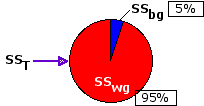
|
As already mentioned, the virtue of the correlated-samples procedure is that it takes the analysis a step further. It has arranged things in advance so that it can identify the portion of SSwg that derives from pre-existing individual differences. And once identified, this portion—in the present case, a very large portion—can be removed. The details of identification and removal will be described in Part 2.
End of Chapter 15, Part 1.
Return to Top of Chapter 15, Part 1
Go to Chapter 15, Part 2
| Home | Click this link only if the present page does not appear in a frameset headed by the logo Concepts and Applications of Inferential Statistics |