©Richard Lowry, 1999-
All rights reserved.
Chapter 15.
One-Way Analysis of Variance for Correlated Samples
Part 2
| A [0cps] | B [2cps] | C [6cps] | All groups combined
| Na=18 | -∑Xai=466 -∑X2ai= 12800 Ma=25.9 SSa=735.8 Nb=18 | -∑Xbi=485 -∑X2bi= 14021 Mb=26.9 SSb=952.9 Nc=18 | -∑Xci=421 -∑X2ci= 10443 Mc=23.4 SSc=596.3 NT=54 | -∑XTi=1372 -∑X2Ti= 37264 MT=25.4 SST=2405.0
|
|
SST = 2405.0 | SSwg =TSSa+SSb+SSc = 735.8+952.9+596.3 = 2285.0 SSbg =TSST—SSwg = 2405.0—2285.0 = 120.0 | ||||
¶Identification and Removal of SSsubj
The first five columns of the following table are a somewhat streamlined version of the data table you saw in Part 1. The means for the individual subjects are now highlighted in blue, and next to each subject's mean, in a new column, is a calculation whose general form you will surely recognize from Chapter 14. The difference between each subject's mean and the mean of the total array of data is taken as a deviate:
The square of that difference is accordingly a squared deviate:
And that squared deviate is then weighted by k=3, which is the number of measures (Xai, Xbi, and Xci) on which the subject's mean is based.
It is the same general structure we used in Chapter 14 to calculate the value of SSbg from scratch, to measure the aggregate differences among the k groups. Now what we come out with is SSsubj, which is a measure of the aggregate differences among the 18 individual subjects.
I show you this particular method for calculating SSsubj only because it gives a clear idea of the conceptual structure of the measure. It would not be the method to use for practical computational purposes, as it is likely to end up with a considerable accumulation of rounding error. Also, if you are doing it by hand, it can be rather laborious. The following method is somewhat less laborious and will in any event minimize the risk of rounding errors. You will recognize it as analogous to the computational formula for SSbg that we worked through in Part 1; namely
Except now the string of items to the left of the minus sign is replaced by another string that looks like this:
That is: For each subject in the analysis, take the sum of that subject's scores across all k conditions, square that sum, and then divide the result by k, which is the number of scores on which the sum is based.
Since k is the same for each subject, this portion of the formula to the left of the minus sign can be rewritten as
and the entire formula can then be written more compactly as
The next version of our data table shows the sum for each subject, along with the calculation of the square of each subject's sum.
Recalling that∑XTi=1372 and NT=54, our calculation of SSsubj is accordingly
As always, one must be careful not to get so lost in the calculations as to lose sight of the concepts. What we have just calculated with SSsubj is the amount of variability within the total array of data that derives from individual differences among the subjects. And now that this amount has been identified, it can be removed. The process of removal is one of simple subtraction. The total amount of within-groups variability isSSwg=2285.0. Of this amount, SSsubj=2181.7 is attributal not to sheer, cussed random variability, but to extraneous pre-existing individual differences among the 18 subjects. Remove the latter from the former, and what remains is
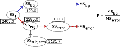
Here is one of the same diagrams you saw in Part 1, except now the specific numerical values have been included for the several values of SS. The bottom line is that a huge chunk of SSwg is attributable to individual differences among the subjects, and that chunk is now removed. From this point on, it is all a smooth ride across familiar terrain.

¶Calculation of MSbg, MSerror, and F
We begin by sorting out the several components of degrees of freedom. The first three are the same as we would have with a one-way independent-samples ANOVA:
The only difference is that now we break dfwg into two further components, corresponding respectively to the two components of within-groups variability, SSsubj and SSerror. For dfsubj the basic concept is once again "the number of items minus one." In this case the number of items is the number of subjects, which we will designate as Nsubj. Thus
Remove this component from dfwg, and what remains is
With these, we can then calculate the two relevant MS values as
and
which in turn give us
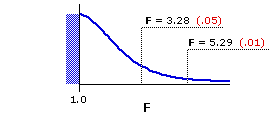
Figure 15.2 shows the sampling distribution of F fordf=2,34, and the adjacent table shows the corresponding portion of Appendix D. As indicated, F=3.28 and F=5.29 mark the points in this distribution beyond which fall 5% and 1%, respectively, of all possible mere-chance outcomes, assuming the null hypothesis to be true.
Figure 15.2. Sampling Distribution of F for df=2,34
ANOVA Summary Table
The assumptions and step-by-step computational procedures for the one-way correlated-samples ANOVA will be outlined in Part 3 of this chapter. It is also in Part 3 that we will see how the Tukey HSD test can be adapted to perform pairwise comparisons among the individual group means in a correlated-samples ANOVA.
| deviate = Msubj* — MT | We will use the subscript "subj*" to mean "any particular subject." The first subject would be subj1; the second, subj2; and so on.
| |
squared deviate = (Msubj* — MT)2
|
| |
weighted squared deviate = k(Msubj* — MT)2
|
| |
| subjects | A | B | C | Subject Means 21 | 22 23 24 25 26 27 28 29 210 211 212 213 214 215 216 217 218
235 | 232 233 232 231 229 229 227 227 228 227 227 224 224 217 217 214 213
239 | 235 232 232 233 230 231 229 231 227 227 226 229 225 216 215 215 213
232 | 231 228 229 226 229 227 227 224 224 223 223 219 219 218 217 212 213
235.3 | 232.7 231.0 231.0 230.0 229.3 229.0 227.7 227.3 226.3 225.7 225.3 224.0 222.7 217.0 216.3 213.7 213.0
3(35.3—25.4)2=294 | 3(32.7—25.4)2=159.9 3(31.0—25.4)2=94.1 3(31.0—25.4)2=94.1 3(30.0—25.4)2=63.5 3(29.3—25.4)2=45.6 3(29.0—25.4)2=38.9 3(27.7—25.4)2=15.9 3(27.3—25.4)2=10.8 3(26.3—25.4)2=2.4 3(25.7—25.4)2=0.3 3(25.3—25.4)2=0 3(24.0—25.4)2=5.9 3(22.7—25.4)2=21.9 3(17.0—25.4)2=211.7 3(16.3—25.4)2=248.4 3(13.7—25.4)2=410.7 3(13.0—25.4)2=461.3 MT=25.4 | SSsubj=2179.4 | | ||||||
I show you this particular method for calculating SSsubj only because it gives a clear idea of the conceptual structure of the measure. It would not be the method to use for practical computational purposes, as it is likely to end up with a considerable accumulation of rounding error. Also, if you are doing it by hand, it can be rather laborious. The following method is somewhat less laborious and will in any event minimize the risk of rounding errors. You will recognize it as analogous to the computational formula for SSbg that we worked through in Part 1; namely
| SSbg | = | (∑Xai)2 Na | + | (∑Xbi)2 Nb | + | (∑Xci)2 Nc | — | (∑XTi)2 NT |
Except now the string of items to the left of the minus sign is replaced by another string that looks like this:
| (∑Xsubj1)2 k | + | (∑Xsubj2)2 k | + | (∑Xsubj3)2 k | + | . . . |
and so on, for as many subjects as you have in the analysis. |
That is: For each subject in the analysis, take the sum of that subject's scores across all k conditions, square that sum, and then divide the result by k, which is the number of scores on which the sum is based.
Since k is the same for each subject, this portion of the formula to the left of the minus sign can be rewritten as
k |
That is: For each subject in the analysis, take the sum of that subject's scores across all k conditions, square that sum, add up these squared sums across all subjects, and then divide the total of squared sums by k. |
and the entire formula can then be written more compactly as
| SSsubj | = | k | — | (∑XTi)2 NT |
The next version of our data table shows the sum for each subject, along with the calculation of the square of each subject's sum.
| subjects | A | B | C | Subject Sums | (∑Xsubj*)2
| 21 | 22 23 24 25 26 27 28 29 210 211 212 213 214 215 216 217 218
235 | 232 233 232 231 229 229 227 227 228 227 227 224 224 217 217 214 213
239 | 235 232 232 233 230 231 229 231 227 227 226 229 225 216 215 215 213
232 | 231 228 229 226 229 227 227 224 224 223 223 219 219 218 217 212 213
2106 | 298 293 293 290 288 287 283 282 279 277 276 272 268 251 249 241 239
1062=11236 | 982=9604 932=8649 932=8649 902=8100 882=7744 872=7569 832=6889 822=6724 792=6241 772=5929 762=5776 722=5184 682=4624 512=2601 492=2401 412=1681 392=1521 | ||||||||
Recalling that
| SSsubj | = | k | — | (∑XTi)2 NT
|
|
| = | 111122 | 3 — | (1372)2 | 54
|
|
| = | 2181.7 | |
As always, one must be careful not to get so lost in the calculations as to lose sight of the concepts. What we have just calculated with SSsubj is the amount of variability within the total array of data that derives from individual differences among the subjects. And now that this amount has been identified, it can be removed. The process of removal is one of simple subtraction. The total amount of within-groups variability is
| SSerror | = SSwg—SSsubj
|
| = 2285.0—2181.7
|
| = 103.3
| |
Here is one of the same diagrams you saw in Part 1, except now the specific numerical values have been included for the several values of SS. The bottom line is that a huge chunk of SSwg is attributable to individual differences among the subjects, and that chunk is now removed. From this point on, it is all a smooth ride across familiar terrain.

¶Calculation of MSbg, MSerror, and F
We begin by sorting out the several components of degrees of freedom. The first three are the same as we would have with a one-way independent-samples ANOVA:
| dfT = NT—1 = 54—1 = 53 | Note that:T dfT = dfbg+dfwg
|
| dfbg = k—1 = 3—1 = 2
|
| and
|
|
| dfwg = NT—k = 54—3 = 51
|
| | |||
dfsubj = Nsubj—1 = 18—1 = 17
|
| |
dferror = dfwg—dfsubj = 51—17 = 34
|
| |
With these, we can then calculate the two relevant MS values as
| MSbg | = | SSbg dfbg | = | 120.0 2 | = 60.0|
| |
| MSerror | = | SSerror dferror | = | 103.3 34 | = 3.0|
| |
| F | = | MSbg MSerror | = | 60.0 3.0 | = 20.0 with df=2,34|
| |
Figure 15.2 shows the sampling distribution of F for
Figure 15.2. Sampling Distribution of F for df=2,34

| |||||||||||||||
| df denomi- nator | df numerator| 1 | 2 | 3 | 34 | 4.13 | 7.44 3.28 | 5.29 2.88 | 4.42
| | ||||||
| As the observed value of | 
|
| Source | SS | df | MS | F | P| between groups | ("effect") 120.0 | 2 | 60.0 | 20.0 | <.01 | within groups | 2285.0 | 51 |
| ·error | 103.3 | 34 | 3.0 | ·subjects | 2181.7 | 17 |
| TOTAL | 2405.0 | 53 | |
The assumptions and step-by-step computational procedures for the one-way correlated-samples ANOVA will be outlined in Part 3 of this chapter. It is also in Part 3 that we will see how the Tukey HSD test can be adapted to perform pairwise comparisons among the individual group means in a correlated-samples ANOVA.
End of Chapter 15, Part 2.
Return to Top of Chapter 15, Part 2
Go to Chapter 15, Part 3
| Home | Click this link only if the present page does not appear in a frameset headed by the logo Concepts and Applications of Inferential Statistics |