For the items covered in Part 2 of this chapter, you will need access to the following summary information from the illustrative analysis performed in Part 1. (Click here if you wish to see the full array of data on which this analysis was performed.)

Ma=28.86

Mb=25.04

Mc=22.50

Md=22.30

Source	SS	df	MS	F	P
between groups ("effect")	140.10	3	46.70	6.42	<.01
within groups ("error")	116.32	16	7.27
TOTAL	256.42	19

---

¶Post-ANOVA Comparisons: the Tukey HSD Test

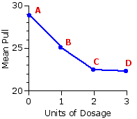A significant F-ratio tells you only that the aggregate difference among the means of the several samples is significantly greater than zero. It does not tell you whether any particular sample mean significantly differs from any particular other. For some research purposes this might be entirely sufficient. Since the investigators in the present example regard their experiment with laboratory rats as only a first step in testing the medication, we can imagine they might be content simply with the global conclusion suggested by the graph of their data: namely, that the curve of "pull" (presumably a reflection of the effect of the medication) slopes downward from A to B to C, then levels off between C and D.

There are, however, many situations in which the investigator might wish to determine specifically whether M_a significantly differs from M_b, or M_b from M_c, and so on. As noted toward the beginning of Chapter 13, this comparison of sample means two at a time cannot be done by way of simple t-tests, because it potentially involves 3 or more comparisons, depending on the number of samples, k, involved in the original analysis. With k=3, there would be 3 potential comparisons:

A·B, A·C, B·C

With k=4, as in the present case, there would be 6 potential comparisons:

A·B, A·C, A·D, B·C, B·D, C·D

With k=5, there would be 10:

A·B, A·C, A·D, A·E, B·C, B·D, B·E, C·D, C·E, D·E

and so forth. The performance of any one or several of these pair-wise comparisons requires a procedure that takes the full range of potential comparisons into account.

The subject of post-ANOVA comparisons is a rather complex one, and most of it lies beyond the scope of an introductory presentation. I will describe here only one of the available procedures, which I think will serve the beginning student well enough for most practical purposes. It goes under the name of the Tukey HSD test, the "HSD" being an acronym for the forthright phrase "honestly significant difference."

The Tukey test revolves around a measure known as the Studentized range statistic, which we will abbreviate as Q. For any particular pair of means among the k groups, let us designate the larger and smaller as M_L and M_S, respectively. The Studentized range statistic can then be calculated for any particular pair as

	Q	=	ML—MS sqrt[MSwg / Np/s]

where MS_wg is the within-groups MS obtained in the original analysis and N_p/s is the number of values of X_i per sample ("p/s"=per sample). For the present example, MS_wg=7.27 and N_p/s=5.

If the k samples are of different sizes, the value of Np/s can be set as equal to the harmonic mean of the sample sizes. For k=3 this would be

Np/s =

3 (1/Na)+(1/Nb)+(1/Nc)

For k=4,

Np/s =

4 (1/Na)+(1/Nb)+(1/Nc)+(1/Nd)

And so on for k=5, k=6, etc.

If the k samples are of different sizes, the value of Np/s can be set as equal to the harmonic mean of the sample sizes. For k=3 this would be

As it happens, you do not really need to worry about calculating Q, because there is a simpler way of applying the Tukey test. However, I will pause to calculate one instance of it, just to give you an idea of what it looks like. For the present example, M_a=28.86, M_b=25.04, MS_wg=7.27, and N_p/s=5. Thus, for the comparison between M_a and M_b the Studentized range statistic would be

	Q	=	28.86—25.04 sqrt[7.27 / 5]	= 3.16

And similarly for any of the other pair-wise comparisons one might wish to make among the means of this particular set of 4 groups.

In any particular case, this Studentized range statistic belongs to a sampling distribution defined by two parameters: the first is k, the number of samples in the original analysis; and the second is df_wg, the number of degrees of freedom associated with the denominator of the F-ratio in the original analysis. Within any particular one of these sampling distributions you can define the value of Q required for significance at any particular level. The following calculator will fetch the critical values of Q at the .05 and .01 levels of significance for any value of K between 3 and 10, inclusive, and for various values of df_wg. To proceed, enter K and df_wg in the designated cells, then click «Calculate». For the present example, with k=4 and df_wg=16, you will end up with Q_.05=4.05 and Q_.01=5.2.

---

Critical Values of Q

k	dfwg		Q.05	Q.01

---

The Tukey HSD test then uses these critical values of Q to determine how large the difference between the means of any two particular groups must be in order to be regarded as significant. The other participants in this determination, MS_wg and N_p/s, are the same items you saw in the earlier formula for Q. The following two "HSD" formulas are simply algebraic jugglings of the original formula, in which the value of Q is set to one or the other of the two critical values, Q_.05 and Q_.01.

For the .05 level:

	HSD.05	=	Q.05 x sqrt	[	MSwg Np/s	]		That is: In order to be considered significant at or beyond the .05 level, the difference between any two particular group means (larger—smaller) must be equal to or greater than 4.88.
		=	4.05 x sqrt	[	7.27 5	]
		=	4.88

And for the .01 level:

	HSD.01	=	Q.01 x sqrt	[	MSwg Np/s	]		That is: In order to be considered significant at or beyond the .01 level, the difference between any two particular group means (larger—smaller) must be equal to or greater than 6.27.
		=	5.2 x sqrt	[	7.27 5	]
		=	6.27

The blue entries in the following table show the differences between each pair of group means in our example. As you can see, two of the comparisons (A·C and A·D) are significant beyond the .01 level, while all the others fail to achieve significance even at the basic .05 level.

	A·B	Ma=28.86 Mb=25.04	3.82	HSD.05 = 4.88 HSD.01 = 6.27
	A·C	Ma=28.86 Mc=22.50	6.36
	A·D	Ma=28.86 Md=22.30	6.56
	B·C	Mb=25.04 Mc=22.50	2.54
	B·D	Mb=25.04 Md=22.30	2.74
	C·D	Mc=22.50 Md=22.30	0.20

Our investigators would therefore be able to conclude that 2 units and 3 units of the experimental medication each produced significantly lower mean levels of "pull" than was found in the zero-unit control group. They would not be able to conclude that the effect of 2 units or 3 units was significantly greater than the effect of 1 unit, nor that the mean "pull" of the 1-unit group was significantly smaller that that of the zero-unit control group. Please note carefully, however, that failing to find a significant difference between M_a and M_b would not entail that 1 unit of the medication has no effect at all. It merely means that the Tukey HSD test does not detect a significant difference between the two in this particular situation. If the investigators had found approximately the same array of group means with samples of twice the size (10 per group, rather than 5), they would very likely have found all of the pair-wise comparisons to be significant, except for the one between M_c and M_d.

---

¶One-Way ANOVA and Correlation

Here yet again is Figure 14.1, which you have now seen several times over. It will be fairly obvious to the naked eye that the two variables, dosage and pull, are correlated in the sense that variations in the one are associated with variations in the other. It will be equally obvious that the relationship is not of the rectilinear (straight-line) sort described in Chapter 3. It is better described by a curved line, hence "curvilinear." Within the context of a one-way analysis of variance for independent samples, a useful measure of the strength of a curvilinear relationship between the independent and dependent variable is given by a quantity known as as eta-square ("eta" to rhyme with "beta"), which is simply the ratio of SS_bg to SS_T. For the medication experiment it comes out as

	eta2	=	SSbg SST	=	140.10 256.42	= 0.55

The essential meaning of "eta²=0.55" is this: Of all the variability that exists within the dependent variable "pull," 55% is associated with variability in the independent variable "dosage level." A moment's reflection of what we observed in Chapter 3 will remind you that this is also the essential meaning of the coefficient of determination, r². The only intrinsic difference between the two is that r² can measure the strength of a correlation only insofar as it is linear (can be described by a straight line), while eta² provides a measure of the strength of correlation irrespective of whether it is linear or curvilinear. If the relationship is linear—fully describable by a straight line—then the values of r² and eta² will be the same. In the degree that a curved line describes the relationship better than a straight line, then eta² will be greater than r².

This point is illustrated by the two panels of Figure 14.3, which show the data for the N_T=20 individual subjects of the experiment laid out in the form of a scatter plot. Applying the procedures of linear correlation to this set of bivariate data will yield the straight regression line shown in the panel on the left, along with r²=0.48. The panel on the right shows the same data with a curvilinear line of best fit, corresponding to our calculated value of eta²=0.55.

Figure 14.3. Linear and Curvilinear Correlation



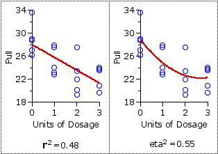
Please note, however, that it is meaningful to speak of eta² as analogous to r² only when the levels of the independent variable are quantitative and linear, as in the present example where zero units, 1 unit, 2 units, and 3 units of the medication represent points along an equal-interval scale. If the levels of the independent variable are only categorical (several different types of medication, several different types of music, etc.), the meaning of eta² reverts back to a version of the more general statement given above: Of all the variability that exists within the dependent variable, such-and-such percent is associated with the differences among the levels of the independent variable.

---

Note that this chapter includes a subchapter on the Kruskal-Wallis Test, which is a non-parametric alternative to the one-way ANOVA for independent samples.