©Richard Lowry, 1999-
All rights reserved.
Chapter 14.
One-Way Analysis of Variance for Independent Samples
Part 1
As most of the logic and procedure for this simplest version of the analysis of variance was developed in Chapter 13, the main portion of the present chapter can be fairly brief and to the point. Part 1 covers the essentials of one-way ANOVA for independent samples. Part 2 touches upon two matters that will take you a bit beyond the bare essentials.
This version of ANOVA applies to the case where you have one independent variable and three or more independent samples of subjects, each sample measured at a different level of the variable. To avoid having to repeat the cumbersome phrase "three or more," we will henceforth refer to the number of independent samples (which is the same as the number of levels of the independent variable) as k. Thus, with three groups of subjects and three levels of the independent variable,k=3; with four groups and four levels, k=4; and so on. We will illustrate the procedure with an example involving k=4.
One of the many complications in the lives of persons who have Alzheimer's disease is that they tend to suffer from frequent periods of intense agitation. Some investigators have theorized that this agitation stems from old aversive conditionings—the conditioned fears and anxieties that a person accumulates over the course of his or her life—with which the Alzheimer's patient is no longer able to cope, on account of severely diminished cognitive capacities.
Against this background, a team of investigators has developed an experimental medication that they believe will substantially decrease the effects of old aversive conditionings. As a preliminary test of the medication, they trained 20 laboratory rats, by standard aversive conditioning procedures, to flee from a certain visual stimulus. These 20 subjects were then randomly and independently sorted intok=4 groups—A, B, C, and D—of 5 subjects each. In the subsequent experimental procedure, the members of each group received via sub-cutaneous injection one or another of four dosage levels of the medication. The members of group A, serving as a control group, received only an inert placebo containing zero units of the medication, while the members of groups B, C, and D received 1 unit, 2 units, and 3 units of the medication, respectively. Five minutes after receiving its injection, each subject was then presented with the aversively conditioned stimulus, and a measure was taken of how hard the subject pulled against a restraining harness in trying to move away from the stimulus. The smaller the pull, the smaller the degree of agitation presumed to be occasioned by the aversive stimulus.
The following table shows the measure of "pull" for each of the 5 subjects in each of the four groups. Also shown are the means of the groups along with MT, the mean of the total array. This table is only our first pass at the data by way of an overview. A fuller listing of summary statistics will be given in a moment.
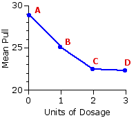
Figure 14.1 provides the same overview in graphical form. Whichever way you look at it, there clearly are differences among the means of the four groups, and these are consistent with what the investigators would have expected if the medication has the effect they suppose it to have. The greatest mean pull, hence presumably the greatest level of agitation, was found with the group that received only the placebo. For the group that received 1 unit of the medication, the mean pull was smaller; and for the groups that received 2 units and 3 units, it was smaller still.
Figure 14.1. Dosage Level and Mean Pull
But of course, here as elsewhere, there is always the possibility that the observed "effect" results from nothing more than mere random variability. And until that possibility is rationally assessed, no conclusions can be drawn, one way or the other. As indicated in Chapter 13, the one-way analysis of variance for independent samples performs that assessment by taking the ratio of two quantities
which is then referred to the appropriate sampling distribution of F, as defined by dfbg and dfwg. For purposes of practical computation, the first step is to calculate the values of∑Xi and ∑X2i for each of the k groups and for all k groups combined. These, in conjunction with the relevant values of N (Na, Nb, etc.), will then permit the calculation of all other quantities required for the analysis. The following table shows the full array of the preliminary summary statistics.
As indicated in the table, the raw measure of variability within the entire array of data, with all k groups combined, isSST=256.42. This, in turn, is composed of two complementary components: SSbg, which is the raw measure of the aggregate differences among the means of the k groups; and SSwg, which is the raw measure of the variability that exists inside the k groups. With k=4, the latter measure comes out as
Assuming that all number-crunching up to this point has been performed without error, you could then calculate the remaining component simply as
However, it is always good practice to check the accuracy of one's calculations by calculating SSbg also from scratch. As you saw in Chapter 13, the weighted squared deviate for each of the k group means can be calculated as
Ng(Mg—MT)2
where Mg is the mean of a particular group and Ng is the number of values of Xi on which that mean is based. Thus, for each of the four groups
An alternative method for calculating SSbg from scratch would be by way of the following computational formula. Although this rather cumbersome-looking device will not provide as clear an idea of the structure of SSbg, it requires fewer computational steps and is also less susceptible to rounding errors.
Here then, in summary, are our two component values of raw variability:
SSbg=140.10 and SSwg=116.32
The next step is to refine them into measures of MS through dividing each by its corresponding number of degrees of freedom. For the between-groups measure, degrees of freedom is the same as outlined in Chapter 13, except now we replace the phrase "number of groups" with the simple designation k.
Similarly for the within-groups measure, except now the groups are notA|B|C but A|B|C|D.
However, once you clearly understand the structure of dfwg, its numerical value can be reached more simply through the algebraically equivalent formula
With the values of SS and df for between-groups and within-groups, we can then calculate
And this, in turn, permits the calculation of theF-ratio as
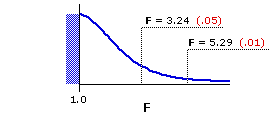
Figure 14.2 shows the sampling distribution of F fordf=3,16. As indicated, F=3.24 and F=5.29 mark the points beyond which fall 5% and 1%, respectively, of all possible mere-chance outcomes, assuming the null hypothesis to be true. These are the same numbers that appear in the table of critical values of F (Appendix D), the relevant portion of which is shown adjacent to the graph.
Figure 14.2. Sampling Distribution of F for df=3,16
As the observed value ofF=6.42 falls to the right of F=5.29, our investigators can regard the aggregate differences among the means of their four samples as significant beyond the .01 level. Recall once again that this term "significant" always has an If/Then logical structure embedded within it, and that the center-point of the structure is always the null hypothesis. For the present example the structure is this: If the null hypothesis were true—if the differences among the means of the four samples were occasioned by nothing more than random variability—then the likelihood of ending up with an F-ratio this large or larger would be less than 1% (P<.01). The investigators can accordingly reject the null hypothesis with a level of confidence somewhat greater than 99%, provisionally concluding that their experimental medication does have the effect they supposed it to have.
ANOVA Summary Tables
When reporting the results of an analysis of variance, it is good practice to present a summary table such as the following. Clearly identifying each component of SS, df, and MS, it allows the reader to take in the main details of the analysis at a single glance.
¶Assumptions of the One-Way ANOVA for Independent Samples
This particular version of the analysis of variance makes the following assumptions about the data that are being fed into it:
t-test for independent samples. The fourth assumption will require a bit of explaining. Listed below are sums of squared deviates within each of our 4 samples. Dividing each by Ng—1 (recall that the subscript "g" means "any particular group") will give an estimate of the variance of the population from which the sample comes. The analysis we have just performed in Part 1 of this chapter assumes that these four variance estimates are all approximately equal. As a practical rule of thumb, you can take the phrase "all approximately equal" to entail that the ratio of the largest sample variance to the smallest should not exceed 1.5.
As you can see, this equal-variance assumption is potentially a bit of bad news. The largest of our sample variances (11.32) is nearly three times as great as the smallest (3.88) and nearly twice as great as the next smallest (5.87). This bad news does not apply only to the present example. It very often happens in real-life applications of ANOVA that sample variances do not satisfy the assumption of being "approximately equal."
But now for the good news. The analysis of variance is a very robust test, in the sense that it is relatively unperturbed when the equal-variance assumption is not met. This is especially so when the k samples are all of the same size, as in the present example. Hence, for this or any other version of ANOVA, it is always a good idea to ensure that all samples are of the same size. (When the several samples are of different sizes, the rule of thumb mentioned above remains in force: the ratio of the largest sample variance to the smallest should not exceed 1.5.)
When the samples are of the same size, the analysis of variance is also robust with respect to the assumption that the source populations are normally distributed. So, in brief, the one-way ANOVA for independent samples can be applied to virtually any set of data that will fit into it, providing that all k of the samples are of equal size and that the first two of the assumptions are met:
¶Step-by-Step Computational Procedure: One-Way Analysis of Variance for Independent Samples
I will show the procedures for the case where the number of groups isk=4. The modifications required for different values of K will be fairly obvious. The steps listed below assume that you have already done the basic number-crunching to get ∑Xi and ∑X2i for each of the k groups and for all k groups combined.
Step 1. Combining all k groups together, calculate
Step 2. For each of the k groups separately, calculate the sum of squared deviates within the group ("g") as
Step 3. Take the sum of the SSg values across all k groups to get
Step 4. Calculate SSbg as
Step 4a. Check your calculations up to this point by calculating SSbg separately as
Step 5. Calculate the relevant degrees of freedom as
Step 6. Calculate the relevant mean-square values as
Step 7. Calculate F as
Step 8. Refer the calculated value of F to the table of critical values of F (Appendix D), with the appropriate pair of numerator/denominator degrees of freedom, as described earlier in this chapter.
This version of ANOVA applies to the case where you have one independent variable and three or more independent samples of subjects, each sample measured at a different level of the variable. To avoid having to repeat the cumbersome phrase "three or more," we will henceforth refer to the number of independent samples (which is the same as the number of levels of the independent variable) as k. Thus, with three groups of subjects and three levels of the independent variable,
One of the many complications in the lives of persons who have Alzheimer's disease is that they tend to suffer from frequent periods of intense agitation. Some investigators have theorized that this agitation stems from old aversive conditionings—the conditioned fears and anxieties that a person accumulates over the course of his or her life—with which the Alzheimer's patient is no longer able to cope, on account of severely diminished cognitive capacities.
Against this background, a team of investigators has developed an experimental medication that they believe will substantially decrease the effects of old aversive conditionings. As a preliminary test of the medication, they trained 20 laboratory rats, by standard aversive conditioning procedures, to flee from a certain visual stimulus. These 20 subjects were then randomly and independently sorted into
The following table shows the measure of "pull" for each of the 5 subjects in each of the four groups. Also shown are the means of the groups along with MT, the mean of the total array. This table is only our first pass at the data by way of an overview. A fuller listing of summary statistics will be given in a moment.
| A 0 units | B 1 unit | C 2 units | D 3 units | Total Array
27.0 | 26.2 28.8 33.5 28.8
22.8 | 23.1 27.7 27.6 24.0
21.9 | 23.4 20.1 27.8 19.3
23.5 | 19.6 23.7 20.8 23.9
| All groups combined.
Ma=28.86
|
Mb=25.04
|
Mc=22.50
|
Md=22.30
|
MT=24.68
| |
Figure 14.1 provides the same overview in graphical form. Whichever way you look at it, there clearly are differences among the means of the four groups, and these are consistent with what the investigators would have expected if the medication has the effect they suppose it to have. The greatest mean pull, hence presumably the greatest level of agitation, was found with the group that received only the placebo. For the group that received 1 unit of the medication, the mean pull was smaller; and for the groups that received 2 units and 3 units, it was smaller still.
Figure 14.1. Dosage Level and Mean Pull
But of course, here as elsewhere, there is always the possibility that the observed "effect" results from nothing more than mere random variability. And until that possibility is rationally assessed, no conclusions can be drawn, one way or the other. As indicated in Chapter 13, the one-way analysis of variance for independent samples performs that assessment by taking the ratio of two quantities
| F = | MSbg MSwg | = | a measure of the aggregate differences among the means of the k groups a measure of the amount of random variability that exists inside the k groups |
which is then referred to the appropriate sampling distribution of F, as defined by dfbg and dfwg. For purposes of practical computation, the first step is to calculate the values of
Units of Dosage| 0 | 1 | 2 | 3 | Total Array
|
27.0 | 26.2 28.8 33.5 28.8
22.8 | 23.1 27.7 27.6 24.0
21.9 | 23.4 20.1 27.8 19.3
23.5 | 19.6 23.7 20.8 23.9
| All groups combined. Na=5 | ∑Xai=144.30 ∑X2ai= 4196.57 Ma=28.86 SSa=32.07 Nb=5 | ∑Xbi=125.20 ∑X2bi= 3158.50 Mb=25.04 SSb=23.49 Nc=5 | ∑Xci=112.50 ∑X2ci= 2576.51 Mc=22.50 SSc=45.26 Nd=5 | ∑Xdi=111.50 ∑X2di= 2501.95 Md=22.30 SSd=15.50 NT=20 | ∑XTi=493.50 ∑X2Ti= 12433.53 MT=24.68 SST=256.42
(If it is not clear where the five values of SS are coming from, click here for an | account of the computational details.) | |||||||
As indicated in the table, the raw measure of variability within the entire array of data, with all k groups combined, is
| SSwg | = SSa+SSb+SSc+SSd|
|
| = 32.07+23.49+45.26+15.50 |
|
| = 116.32 | |
Assuming that all number-crunching up to this point has been performed without error, you could then calculate the remaining component simply as
| SSbg | = SST—SSwg|
|
| = 256.42—116.32 |
|
| = 140.10 | |
However, it is always good practice to check the accuracy of one's calculations by calculating SSbg also from scratch. As you saw in Chapter 13, the weighted squared deviate for each of the k group means can be calculated as
where Mg is the mean of a particular group and Ng is the number of values of Xi on which that mean is based. Thus, for each of the four groups
| A: | 5(28.86—24.68)2 = 87.36 | 140.09 versus 140.10. Close enough. The slight difference between the two derives from rounding errors in the present calculation. (Each mean value starts out rounded to two decimal places.) | |||||||||
| B: | 5(25.04—24.68)2 = 0.65
|
| C:
| 5(22.50—24.68)2 = 23.76
|
| D:
| 5(22.30—24.68)2 = 28.32
|
|
| SSbg = 140.09 |
An alternative method for calculating SSbg from scratch would be by way of the following computational formula. Although this rather cumbersome-looking device will not provide as clear an idea of the structure of SSbg, it requires fewer computational steps and is also less susceptible to rounding errors.
| SSbg | = | (∑Xai)2 Na | + | (∑Xbi)2 Nb | + | (∑Xci)2 Nc | + | (∑Xdi)2 Nd | — | (∑XT)2 NT
|
|
| = | (144.3)2 | 5 + | (125.2)2 | 5 + | (112.5)2 | 5 + | (111.5)2 | 5 — | (493.5)2 | 20
|
|
| = | 140.10 | |
Here then, in summary, are our two component values of raw variability:
The next step is to refine them into measures of MS through dividing each by its corresponding number of degrees of freedom. For the between-groups measure, degrees of freedom is the same as outlined in Chapter 13, except now we replace the phrase "number of groups" with the simple designation k.
| dfbg | = k—1|
|
| = 4—1 = 3 | |
Similarly for the within-groups measure, except now the groups are not
| dfwg | = (Na—1)+(Nb—1)+(Nc—1)+(Nd—1)|
|
| = (5—1)+(5—1)+(5—1)+(5—1) = 16 | |
However, once you clearly understand the structure of dfwg, its numerical value can be reached more simply through the algebraically equivalent formula
| dfwg | = NT—k|
|
| = 20—4 = 16 | |
Note that dfT, the number of degrees of freedom for the entire array of data, is dfT = 20—1 = 19 and that dfbg+dfwg=dfT. |
With the values of SS and df for between-groups and within-groups, we can then calculate
| MSbg | = | SSbg dfbg | = | 140.10 3 | = 46.70| and |
| MSwg | = | SSwg | dfwg = | 116.32 | 16 = 7.27 | | ||
And this, in turn, permits the calculation of the
| F | = | MSbg MSwg | = | 46.70 7.27 | = 6.42 with df=3,16 |
Figure 14.2 shows the sampling distribution of F for
Figure 14.2. Sampling Distribution of F for df=3,16
| |||||||||||||||
| df denomi- nator | df numerator| 1 | 2 | 3 | 16 | 4.49 | 8.53 3.63 | 6.23 3.24 | 5.29
| | ||||||
As the observed value of
It is possible to calculate the probability associated with an |
When reporting the results of an analysis of variance, it is good practice to present a summary table such as the following. Clearly identifying each component of SS, df, and MS, it allows the reader to take in the main details of the analysis at a single glance.
| Source | SS | df | MS | F | P| between groups | ("effect") 140.10 | 3 | 46.70 | 6.42 | <.01* | within groups | ("error") 116.32 | 16 | 7.27 | TOTAL | 256.42 | 19 | |
|
*As indicated above, the probability value for this analysis could also be reported as P=.005. |
¶Assumptions of the One-Way ANOVA for Independent Samples
This particular version of the analysis of variance makes the following assumptions about the data that are being fed into it:
- that the scale on which the dependent variable is measured has the properties of an equal interval scale;
- that the k samples are independently and randomly drawn from the source population(s);
- that the source population(s) can be reasonably supposed to have a normal distribution; and
- that the k samples have approximately equal variances.
| Group | SS | Ng—1 | Variance Estimate A | 32.07 | 4 | 8.02 | B | 23.49 | 4 | 5.87 | C | 45.26 | 4 | 11.32 | D | 15.50 | 4 | 3.88 | |
But now for the good news. The analysis of variance is a very robust test, in the sense that it is relatively unperturbed when the equal-variance assumption is not met. This is especially so when the k samples are all of the same size, as in the present example. Hence, for this or any other version of ANOVA, it is always a good idea to ensure that all samples are of the same size. (When the several samples are of different sizes, the rule of thumb mentioned above remains in force: the ratio of the largest sample variance to the smallest should not exceed 1.5.)
When the samples are of the same size, the analysis of variance is also robust with respect to the assumption that the source populations are normally distributed. So, in brief, the one-way ANOVA for independent samples can be applied to virtually any set of data that will fit into it, providing that all k of the samples are of equal size and that the first two of the assumptions are met:
- that the scale on which the dependent variable is measured has the properties of an equal interval scale; and
- that the k samples are independently and randomly drawn from the source population(s).
¶Step-by-Step Computational Procedure: One-Way Analysis of Variance for Independent Samples
I will show the procedures for the case where the number of groups is
Step 1. Combining all k groups together, calculate
| SST = ∑X2i — | (∑Xi)2 NT |
Step 2. For each of the k groups separately, calculate the sum of squared deviates within the group ("g") as
| SSg = ∑X2gi — | (∑Xgi)2 Ng |
Step 3. Take the sum of the SSg values across all k groups to get
| SSwg = SSa+SSb+SSc+SSd |
Step 4. Calculate SSbg as
| SSbg = SST—SSwg |
Step 4a. Check your calculations up to this point by calculating SSbg separately as
| SSbg | = | (∑Xai)2 Na | + | (∑Xbi)2 Nb | + | (∑Xci)2 Nc | + | (∑Xdi)2 Nd | — | (∑XT)2 NT |
Step 5. Calculate the relevant degrees of freedom as
dfT = NT—1|
| dfbg = k—1 |
| dfwg = NT—k | |
Step 6. Calculate the relevant mean-square values as
| MSbg | = | SSbg dfbg and |
| MSwg | = | SSwg | dfwg | ||
Step 7. Calculate F as
| F | = | MSbg MSwg |
Step 8. Refer the calculated value of F to the table of critical values of F (Appendix D), with the appropriate pair of numerator/denominator degrees of freedom, as described earlier in this chapter.
End of Chapter 14, Part 1.
Return to Top of Chapter 14, Part 1
Go to Chapter 14, Part 2
| Home | Click this link only if the present page does not appear in a frameset headed by the logo Concepts and Applications of Inferential Statistics |