©Richard Lowry, 1999-
All rights reserved.
Chapter 9.
Introduction to Procedures Involving Sample Means
Part 3
From Chapter 9, Part 2:T
William S. Gosset's notable achievement was the mathematical discovery that, even thought-ratios are based on estimates, they nonetheless behave in a precise, orderly fashion. Specifically, what he discovered was that when t-ratios are considered en masse they form relative-frequency distributions whose outlines are capable of being precisely known; and further, that this precise knowledge of the outlines can then be used as a basis for making precise probability judgments, in much the same way that precise knowledge of the properties of the normal distribution permits us to make precise probability assessments in connection with z-ratios.
To illustrate this point, let us return for a moment to the reference source population introduced in Part 1 of this chapter.
Figure 9.1 [repeated]. Reference Source Population, Normally Distributed with =18 and
  =±3
=±3

Suppose we were to draw a vast number of pairs of random samples from this population, each sample of size N=10. Since this is a source population for which we know the true values ofi 2
2 and i ,
, we could easily calculate a proper z-ratio for each pair. If we were then to take all these z-ratios and lay them out in the form of a frequency distribution, we would find that it very closely approximates the shape of the unit normal distribution. That, in fact, is precisely why it is meaningful to refer a z-ratio to the table of the unit normal distribution.
But now let us go back to the very same pairs of samples and calculatet-ratios for them. That is, for each pair of samples we separately calculate the ratio
If we were then to take all these t-ratios and lay them out in the form of a frequency distribution, they too would form an orderly, symmetrical outline. It would not be a normal distribution—not in this particular case, anyway—but orderly all the same, and equally useful for making precise probability judgments. Figure 9.4 shows what these two distributions of z and t would look like. The most readily visible difference between them is that the t-distribution is somewhat flatter and more spread out. The implication is that values of t that lie toward the center of the distribution are somewhat less probable than comparable values of z, while those that lie toward the extremes are somewhat more probable than comparable values of z.
Figure 9.4. The Unit Normal Distribution Compared with thet-Distribution for df=18

Another difference between the distributions of z and t is that, while there is one and only one unit normal distribution, there is a whole range of differentt-distributions. Indeed, there is a separate t-distribution for each possible value of degrees of freedom. The concept of degrees of freedom in the present context is much the same as the one introduced in Chapter 8 in connection with chi-square procedures. Essentially, it is an index of the amount of random variability that can be present in the particular situation. If you have a single sample of size N, the number of degrees of freedom is
df = N—1
If you have two samples of sizes Na and Nb, it is
df = (Na—1)+(Nb—1)
In the present case we have two samples of sizes Na=10 and Nb=10, so the number of degrees of freedom is (10—1)+(10—1)=18.
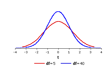
The general pattern of resemblances and differences among the various t-distributions is illustrated in Figure 9.5, which shows the distributions of t for df=5 and df=40.
Figure 9.5. The Distributions of t for df=5 and df=40

Notice that the t-distribution for df=5 is even flatter and more spread out than the one shown in Figure 9.4 for df=18, whereas the one for df=40 is markedly less flat and spread out. Indeed, to the naked eye thet-distribution for df=40 is scarcely distinguishable from the normal distribution. It is also a very close fit mathematically. In general, the smaller the number of degrees of freedom, the greater the difference between the corresponding t-distribution and the unit normal distribution. Conversely, the larger the number of degrees of freedom, the more closely the corresponding t-distribution will approximate the unit normal distribution.
The logic of probability assessment is the same witht-distributions as with the unit normal distribution. The probability of getting a result "this large or larger" is equal to the proportion of the distribution that lies to the right (+) or left (—) of the calculated value of t, depending of the direction of the hypothesis the researcher is seeking to test. For a non-directional two-way hypothesis it is the total proportion that lies both to the right of +t and to the left of —t. The full table of critical values of t can be found in Appendix C. The abbreviated version shown below will give you an idea of how it is laid out.
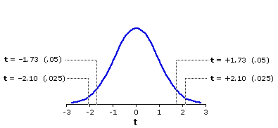
To the right of each value of df are the values of+t or —t that must be met or exceeded in order for a result to be significant at or beyond a particular level of significance. To illustrate, note that the first two values lying to the right of df=18 are 1.73 and 2.10. These and the other values in that row (2.55, 2.88, 3.92) refer to specific locations within the sampling distribution of t for the case where degrees of freedom is equal to 18. As shown graphically in Figure 9.6, t=+1.73 marks the point in this distribution beyond which (to the right, away from the mean) falls 5% of the total area of the distribution. An obtained t-ratio equal to or greater than +1.73 is accordingly significant at or beyond the .05 level for a directional ("one-tailed") test. (The distinction between directional and non-directional tests of significance is introduced in Chapter 7.)
Figure 9.6. Sampling Distribution of t for df=18

I began this portion of the chapter by asking you to suppose you we were drawing a vast number of pairs of random samples from our reference source population, calculating thet-ratio for each pair. The following demonstration gives you the opportunity to do exactly that, and in the process to decide for yourself whether all this talk about the sampling distributions of t has any basis in reality. Each time you click the button, your computer will draw ten pairs of random samples. For each pair, Na=10, Nb=10, hence df=18. Whenever the t-ratio produced by a pair falls at or beyond the 5% level at either end of the df=18 sampling distribution (t<—1.73 on the left or t>+1.73 on the right), it will be marked as "***". Click the button thirty or forty times and you will find the cumulative proportion of these cases coming very close to the theoretical proportion of 5%+5%=10%. The average batch of ten sample pairs will therefore include one t-ratio marked as "***", although any particular batch might of course have more than one or none at all.
In the next three chapters we will examine the eminently practical applications to which all this abstract theorizing can be put. Meanwhile, note that the present chapter includes an Appendix that will generate a graphic and numerical display of the properties of the sampling distribution of t for any value of df between 4 and 200, inclusive. As the page opens, you will be prompted to enter the value of df.
| t-ratio for comparing the mean of a sample with the mean (either actual or hypothetical) of a population: |
| t = | MX— est.:
| | |||
| t-ratio for comparing the means of a two samples: |
| t = | MXa—MXb est.:
| | |||
William S. Gosset's notable achievement was the mathematical discovery that, even though
To illustrate this point, let us return for a moment to the reference source population introduced in Part 1 of this chapter.
Figure 9.1 [repeated]. Reference Source Population, Normally Distributed with

Suppose we were to draw a vast number of pairs of random samples from this population, each sample of size N=10. Since this is a source population for which we know the true values of
But now let us go back to the very same pairs of samples and calculate
| t = | MXa—MXb est.: |
If we were then to take all these t-ratios and lay them out in the form of a frequency distribution, they too would form an orderly, symmetrical outline. It would not be a normal distribution—
Figure 9.4. The Unit Normal Distribution Compared with the

Another difference between the distributions of z and t is that, while there is one and only one unit normal distribution, there is a whole range of different
df = N—1
If you have two samples of sizes Na and Nb, it is
df = (Na—1)+(Nb—1)
In the present case we have two samples of sizes Na=10 and Nb=10, so the number of degrees of freedom is (10—1)+(10—1)=18.
The general pattern of resemblances and differences among the various t-distributions is illustrated in Figure 9.5, which shows the distributions of t for df=5 and df=40.
Figure 9.5. The Distributions of t for df=5 and df=40

Notice that the t-distribution for df=5 is even flatter and more spread out than the one shown in Figure 9.4 for df=18, whereas the one for df=40 is markedly less flat and spread out. Indeed, to the naked eye the
The logic of probability assessment is the same with
Level of Significance| df | 5 10 18 20 .05 | --- 2.02 1.81 1.73 1.72 .025 | .05 2.57 2.23 2.10 2.09 .01 | .02 3.36 2.76 2.55 2.53 .005 | .01 4.03 3.17 2.88 2.85 .0005 | .001 6.87 4.59 3.92 3.85 directional test | non-directional test | ||||||||||||||
To the right of each value of df are the values of
Figure 9.6. Sampling Distribution of t for df=18

| Similarly, t=+2.10 marks the point beyond which falls 2.5% of the distribution, so an obtained | For a non-directional ("two-tailed") test, the probability associated with an obtained value of t is twice that associated with the same value of t for a directional test. Thus, for a non-directional test with |
I began this portion of the chapter by asking you to suppose you we were drawing a vast number of pairs of random samples from our reference source population, calculating the
In the next three chapters we will examine the eminently practical applications to which all this abstract theorizing can be put. Meanwhile, note that the present chapter includes an Appendix that will generate a graphic and numerical display of the properties of the sampling distribution of t for any value of df between 4 and 200, inclusive. As the page opens, you will be prompted to enter the value of df.
End of Chapter 9.
Return to Top of Chapter 9, Part 3
Go to Chapter 10 [t-Procedures for Estimating the Mean of a Population]
| Home | Click this link only if the present page does not appear in a frameset headed by the logo Concepts and Applications of Inferential Statistics |