©Richard Lowry, 1999-
All rights reserved.
Chapter 10.
t-Procedures for Estimating the Mean of a Population
An archeologist has found 19 intact specimens of a certain prehistoric artifact. Although she finds the specimens individually interesting in and of themselves, her broader research interest is in what they can tell her about the entire population of such artifacts that must once have existed within this particular prehistoric setting. As a first step she undertakes, on the basis of information contained within her sample, to estimate the mean length of such artifacts within the population. Listed below are the lengths of the 19 items in the sample, each measured to the nearest tenth of a centimeter. Also shown are the mean of the sample, the sum of squared deviates, the variance, and the standard deviation.
We noted in Chapter 9 that the mean of a sample can be taken as an unbiased estimate of the mean of the population from which it is randomly drawn. Our archeologist is of course well aware that her sample of N=19 was not actively "drawn" from the population; it is simply the 19 specimens that happen to have been found intact. It is, however, commonly recognized within her field that the survival and discovery of intact artifacts of this particular provenience is a matter of the merest chance, so she considers it reasonable to assume that the sample, though not actively drawn, is nonetheless random and therefore an unbiased representation of the population. Having found nothing in the texture of her data to suggest anything to the contrary, she is also prepared to assume that the source population is normally distributed. Providing that these two assumptions are correct, she can then conclude that the mean of the population must lie somewhere in the vicinity of the observed mean of the sample. Thus, following the general formulaic structure introduced in Chapter 9
All that now remains is to work out the details for the portion of this structure that reads "±[definition of 'vicinity']." We will first develop the underlying logic of the procedure, and then translate this logic into the nuts-and-bolts of practical application.
¶The Underlying Logic
This is another of those "if only" scenarios: If only we knew in advance the variability of the population from which the sample comes. For the sake of illustration, suppose for a moment that the measures of variability found within the sample could be taken as the true, precise measures of variance and standard deviation within the entire population. In fact, they cannot be taken this way; but suppose just for the moment that they could. This would give us
Where we go from here must be prefaced with a reminder of three points developed in Chapter 9:
which in the present case would yield
As shown in Figure 10.1, this would entail that the mean of the sample belongs to a sampling distribution in which each unit of standard deviation is equal to 0.83 units of the original scale of measurement.
Figure 10.1. Sampling Distribution of the Means of Samples of Size N=19 Randomly Drawn from a Normally Distributed Source Population with source=±3.6
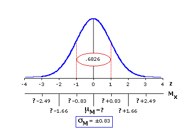
The meaning of the red-bordered ellipse in the center of the distribution will be fairly obvious by now. As we have noted on several previous occasions, 68.26% of all the constituents of a normal distribution (in the present case, the constituents are sample means) fall within one standard deviation of the distribution's mean. We of course do not know what the mean of the distribution is—but, whatever it might be, we know that any particular randomly selected constituent has a 68.26% chance of falling within ±1 standard deviation of it.
The next step is to recognize the symmetry of this relationship. If the mean of any particular sample has a 68.26% chance of falling within ±1 standard deviation of the distribution's mean, then the distribution's mean has an identical 68.26% chance of falling within ±1 standard deviation of the mean of any particular sample. In the present case the observed mean of the sample is MX=18.9 and the calculated value of the standard deviation of the sampling distribution isi M=±0.83. So our investigator can be 68.26% confident that the true mean of the sampling distribution, hence the true mean of the source population, lies somewhere within ±0.83 centimeters of 18.9; that is, between 18.08cm and 19.73cm, inclusive. A procedure of this general type is typically spoken of as a point and interval estimation. "Point" refers to the estimated location of the mean of the source population, and "interval" denotes the plus-or-minus range around this point that defines the concept of "somewhere in the vicinity." This latter is also spoken of as the confidence interval. In the present example the "point" is 18.9cm and the 68.26% confidence interval extends ±0.83cm on either side of that point.
Expressing it formulaically, our archeologist could therefore conclude with 68.26% confidence that
I have begun with this example of the 68.26% level of confidence only because its connection with ±1 standard deviation makes it easy to grasp intuitively. In actual scientific work the preference is usually for the more stringent 95% level, sometimes for the even stricter 99% level. The next version of Figure 10.1 shows the details of the sampling distribution for this scenario that would pertain to the 95% confidence level.
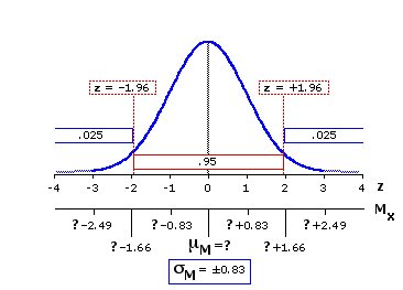
In the table of the normal distribution (Appendix A) you will find that 2.5% of the distribution falls to the left ofz=—1.96 and an equivalent 2.5% falls to the right of z=+1.96. The obvious implication is that the remaining 95% of the distribution lies between z=—1.96 and z=+1.96. It is the same logic as before, but with a somewhat different cast of characters. Any particular randomly selected constituent of the distribution has a 95% chance of falling within ±1.96 standard deviations of the distribution's mean. Symmetrically, there is a 95% chance that the mean of the distribution will lie within ±1.96 standard deviations of any particular randomly selected constituent. Recalling that each unit of z in the present case corresponds to 0.83cm on the original scale of measurement, our point and interval estimate for the 95% confidence level would accordingly be
The final version of Figure 10.1 shows the details pertaining to the 99% confidence level.
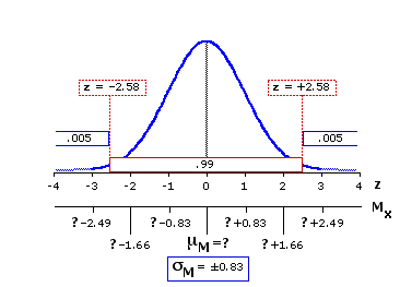
Here the critical value of z is ±2.58. To the left ofz=—2.58 falls one-half of one percent of the distribution; an equivalent one-half of one percent falls to the right of z=+2.58; and the remaining 99% lies between these two markers. So our point and interval estimate for the 99% confidence level would be
¶The Practical Application
I began the foregoing section by asking you to suppose that the measures of variability found within the sample could be taken as the true, precise measures of variance and standard deviation within the entire source population. This assumption is of course completely untenable, for in reality it is highly unlikely that the variability of any particular sample would be identical with that of the population. However, as spelled out in Chapter 9, the variability observed within the sample does provide a basis for rationally and systematically estimating the variability of the source population. Beyond this, the only difference between the procedure outlined above and the one we will now examine is the difference between z and t. When the variability of the source population is known only through estimation, the sampling distribution to which you ultimately refer is one or another of the distributions of t. For the present example, it is thet-distribution pertaining to df=18 (recall that for a single sample, df=N—1).
To refresh your memory of details, here again are the N=19 measures of length observed by our archeologist, along with their mean and sum of squared deviates.
As described in Chapter 9, the variance of the source population can be estimated as
That, in turn, allows us to estimate the standard deviation of the sampling distribution of sample means as
The following abbreviated table lists the critical values of t for df=18 (for the full table see Appendix C), and Figure 10.2 below it shows in graphic form the sampling distribution to which these values refer. Note in particular the two critical values listed in red.
Figure 10.2. Sampling Distribution of t for df=18
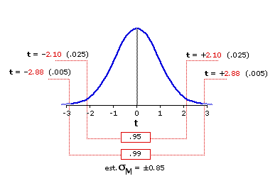
For the next step we do exactly what we did earlier with z, except now the reference is to t. In the sampling distribution of t for df=18, 95% of the distribution falls within ±2.10 units of t from the mean. Given that each unit of t in this case is equal to 0.85 units on the original scale of measurement, the estimate of the source population's mean for the 95% level of confidence would be
And similarly for the 99% level of confidence. In the sampling distribution of t for df=18, 99% of the distribution falls within ±2.88 units of t from the mean. Hence
Our archeological researcher could therefore estimate with 99% confidence that the true mean of the population from which her sample comes lies somewhere between 16.45cm and 21.35cm, inclusive. If she were willing to settle for the 95% level of confidence, she could narrow that range down to between 17.11cm and 20.69cm, inclusive.
¶Step-by-Step Computational Procedure for Estimating the Mean of a Population on the Basis of Information Contained within a Sample
Step 1. For the sample of N values of Xi, calculate
Step 2. Estimate the variance of the source population as
Step 3. Estimate the standard deviation of the sampling distribution of sample means (the "standard error" of the mean) as
Step 4. Perform the point and interval estimate as
with df=N—1.
For the 95% confidence level, tcritical is the value of t that is listed in the conventional table of t as significant at the .05 level for a non-directional ("two-tailed") test. For the 99% confidence level, it is the value listed as significant at the .01 level for a non-directional test. In the following abbreviated version of the table of t, the values of tcritical for the 95% and 99% confidence levels are listed in blue and red, respectively. The particular value of tcritical employed would of course depend on the relevant value of df. The full table of t can be found in Appendix C.
When you perform a point and interval estimate at the 95% confidence level, the implication is that you have a 95% chance of being right and a 5% chance of being wrong. Similarly for an estimate at the 99% level: you have a 99% chance of being right and a 1% chance of being wrong. It all sounds fine in principle, but would it really work out that way in practice? I hope the following demonstration will help to convince you that it would.
Each time you click the button labeled "Sample," your computer will perform a 95% point and interval estimate based on a sample of size N=19 randomly drawn from the reference source population described in Chapter 9. As in the archeological example above, degrees of freedom is 18 and tcritical for the 95% confidence levelis ±2.10. So the calculation for each sample will take the form
est. source = MX ±(2.10 x est.
 M)
M)
In this particular situation we know the true mean of the population to be
i source = 18.0
so it will be determinable in each instance whether the estimate is right or wrong. The estimate is "right" when the true mean of the population lies within the calculated 95% confidence interval, and it is "wrong" when the true population mean falls outside that interval. Each right estimate will be marked by a blue square next to it, and each wrong one by a red square. If you click the button a sufficiently large number of times, you will find the percentage of right estimates closely approximating the theoretical value of 95%. However, even as few as twenty or thirty clicks should make it clear that all but a few of such estimates will in fact include the true mean of the population within their specified plus-or-minus range. (If red squares turn up fairly frequently at the outset, keep in mind that there is always the possibility of ending up with something improbable and extraordinary within any particular small set of samples. Keep clicking several hundred times over, and you will see the proportions of right and wrong estimates closely approximating 0.95 and 0.05, respectively.)
17.3, 18.9, 17.7, 23.8, 16.0 22.1, 18.4, 18.2, 13.3, 26.8 18.6, 24.5, 22.8, 13.4, 18.1 14.8, 20.6, 17.4, 16.1 | MX = 18.9 SS = 248.5 s2 = 248.5/19 = 13.1 s = sqrt[13.1] = ±3.6 |
We noted in Chapter 9 that the mean of a sample can be taken as an unbiased estimate of the mean of the population from which it is randomly drawn. Our archeologist is of course well aware that her sample of N=19 was not actively "drawn" from the population; it is simply the 19 specimens that happen to have been found intact. It is, however, commonly recognized within her field that the survival and discovery of intact artifacts of this particular provenience is a matter of the merest chance, so she considers it reasonable to assume that the sample, though not actively drawn, is nonetheless random and therefore an unbiased representation of the population. Having found nothing in the texture of her data to suggest anything to the contrary, she is also prepared to assume that the source population is normally distributed. Providing that these two assumptions are correct, she can then conclude that the mean of the population must lie somewhere in the vicinity of the observed mean of the sample. Thus, following the general formulaic structure introduced in Chapter 9
| est. | = MX±[definition of 'vicinity']
|
|
| = 18.9±[definition of 'vicinity']
| |
All that now remains is to work out the details for the portion of this structure that reads "±[definition of 'vicinity']." We will first develop the underlying logic of the procedure, and then translate this logic into the nuts-and-bolts of practical application.
¶The Underlying Logic
This is another of those "if only" scenarios: If only we knew in advance the variability of the population from which the sample comes. For the sake of illustration, suppose for a moment that the measures of variability found within the sample could be taken as the true, precise measures of variance and standard deviation within the entire population. In fact, they cannot be taken this way; but suppose just for the moment that they could. This would give us
i i | Hypothetical. For illustrative purposes only. Don't do it this way in practice. |
Where we go from here must be prefaced with a reminder of three points developed in Chapter 9:
| (1) | If the source population is normally distributed, then so, too, will be the sampling distribution of sample means.
| (2)
| The mean of the sampling distribution will be equal to the mean of the source population:i | i So if we can figure out the value ofi (3)
| When the variability of the source population is precisely known (in the present case it actually is not, but we are pretending for the moment that it is), the standard deviation of the sampling distribution can be calculated directly as:
| |
| i | = | sqrt[N] | From Ch.9, Pt.1. | |||
which in the present case would yield
| i | = | ±3.6 sqrt[19] | = ±0.83 |
As shown in Figure 10.1, this would entail that the mean of the sample belongs to a sampling distribution in which each unit of standard deviation is equal to 0.83 units of the original scale of measurement.
Figure 10.1. Sampling Distribution of the Means of Samples of Size N=19 Randomly Drawn from a Normally Distributed Source Population with

The meaning of the red-bordered ellipse in the center of the distribution will be fairly obvious by now. As we have noted on several previous occasions, 68.26% of all the constituents of a normal distribution (in the present case, the constituents are sample means) fall within one standard deviation of the distribution's mean. We of course do not know what the mean of the distribution is—
The next step is to recognize the symmetry of this relationship. If the mean of any particular sample has a 68.26% chance of falling within ±1 standard deviation of the distribution's mean, then the distribution's mean has an identical 68.26% chance of falling within ±1 standard deviation of the mean of any particular sample. In the present case the observed mean of the sample is MX=18.9 and the calculated value of the standard deviation of the sampling distribution isi
Expressing it formulaically, our archeologist could therefore conclude with 68.26% confidence that
| est. | = MX ±|
|
| = 18.9±0.83
| |
I have begun with this example of the 68.26% level of confidence only because its connection with ±1 standard deviation makes it easy to grasp intuitively. In actual scientific work the preference is usually for the more stringent 95% level, sometimes for the even stricter 99% level. The next version of Figure 10.1 shows the details of the sampling distribution for this scenario that would pertain to the 95% confidence level.

In the table of the normal distribution (Appendix A) you will find that 2.5% of the distribution falls to the left of
| est. | = MX ±(1.96 x|
|
| = 18.9±(1.96 x 0.83)
|
|
| = 18.9±1.63
| |
The final version of Figure 10.1 shows the details pertaining to the 99% confidence level.

Here the critical value of z is ±2.58. To the left of
| est. | = MX ±(2.58 x|
|
| = 18.9±(2.58 x 0.83)
|
|
| = 18.9±2.14
| |
¶The Practical Application
I began the foregoing section by asking you to suppose that the measures of variability found within the sample could be taken as the true, precise measures of variance and standard deviation within the entire source population. This assumption is of course completely untenable, for in reality it is highly unlikely that the variability of any particular sample would be identical with that of the population. However, as spelled out in Chapter 9, the variability observed within the sample does provide a basis for rationally and systematically estimating the variability of the source population. Beyond this, the only difference between the procedure outlined above and the one we will now examine is the difference between z and t. When the variability of the source population is known only through estimation, the sampling distribution to which you ultimately refer is one or another of the distributions of t. For the present example, it is the
To refresh your memory of details, here again are the N=19 measures of length observed by our archeologist, along with their mean and sum of squared deviates.
17.3, 18.9, 17.7, 23.8, 16.0 22.1, 18.4, 18.2, 13.3, 26.8 18.6, 24.5, 22.8, 13.4, 18.1 14.8, 20.6, 17.4, 16.1 | MX = 18.9 SS = 248.5 |
| {s2} | = | SS N—1 | estimate of: From Ch.9, Pt.2
|
|
| =
| 248.5 | 18 = 13.81
| | |||
That, in turn, allows us to estimate the standard deviation of the sampling distribution of sample means as
| est. | = | sqrt | [ | {s2} N | ] | From Ch.9, Pt.2
|
|
| = | sqrt | [
| 13.81 | 19 ]
| = ±0.85 | | |||
The following abbreviated table lists the critical values of t for df=18 (for the full table see Appendix C), and Figure 10.2 below it shows in graphic form the sampling distribution to which these values refer. Note in particular the two critical values listed in red.
Level of Significance| df | 18 .05 | --- 1.73 .025 | .05 2.10 .01 | .02 2.55 .005 | .01 2.88 .0005 | .001 3.92 directional test | non-directional test | ||||||||||||||
Figure 10.2. Sampling Distribution of t for df=18

For the next step we do exactly what we did earlier with z, except now the reference is to t. In the sampling distribution of t for df=18, 95% of the distribution falls within ±2.10 units of t from the mean. Given that each unit of t in this case is equal to 0.85 units on the original scale of measurement, the estimate of the source population's mean for the 95% level of confidence would be
| est. | = MX ±(2.10 x est.|
|
| = 18.9±(2.10 x 0.85)
|
|
| = 18.9±1.79
| |
And similarly for the 99% level of confidence. In the sampling distribution of t for df=18, 99% of the distribution falls within ±2.88 units of t from the mean. Hence
| est. | = MX ±(2.88 x est.|
|
| = 18.9±(2.88 x 0.85)
|
|
| = 18.9±2.45
| |
Our archeological researcher could therefore estimate with 99% confidence that the true mean of the population from which her sample comes lies somewhere between 16.45cm and 21.35cm, inclusive. If she were willing to settle for the 95% level of confidence, she could narrow that range down to between 17.11cm and 20.69cm, inclusive.
¶Step-by-Step Computational Procedure for Estimating the Mean of a Population on the Basis of Information Contained within a Sample
Note that this process makes the following assumptions and can be meaningfully applied only insofar as these assumptions are met:
That the scale of measurement has the properties of an equal interval scale.
That the sample is randomly drawn from the source population.
That the source population can be reasonably supposed to have a normal distribution.
Step 1. For the sample of N values of Xi, calculate
| MX | the mean of the sample
| SS
|
| the sum of squared deviates |
Step 2. Estimate the variance of the source population as
| {s2} | = | SS N—1 |
Step 3. Estimate the standard deviation of the sampling distribution of sample means (the "standard error" of the mean) as
| est. | = | sqrt | [ | {s2} N | ] |
Note that Steps 2 and 3 can be combined into the more streamlined formula
| est. | = | sqrt | [ | SS/(N—1) N | ] |
Step 4. Perform the point and interval estimate as
| est. |
with df=N—1.
For the 95% confidence level, tcritical is the value of t that is listed in the conventional table of t as significant at the .05 level for a non-directional ("two-tailed") test. For the 99% confidence level, it is the value listed as significant at the .01 level for a non-directional test. In the following abbreviated version of the table of t, the values of tcritical for the 95% and 99% confidence levels are listed in blue and red, respectively. The particular value of tcritical employed would of course depend on the relevant value of df. The full table of t can be found in Appendix C.
Level of Significance| df | 5 10 18 20 .05 | --- 2.02 1.81 1.73 1.72 .025 | .05 2.57 2.23 2.10 2.09 .01 | .02 3.36 2.76 2.55 2.53 .005 | .01 4.03 3.17 2.88 2.85 .0005 | .001 6.87 4.59 3.92 3.85 directional test | non-directional test | ||||||||||||||
When you perform a point and interval estimate at the 95% confidence level, the implication is that you have a 95% chance of being right and a 5% chance of being wrong. Similarly for an estimate at the 99% level: you have a 99% chance of being right and a 1% chance of being wrong. It all sounds fine in principle, but would it really work out that way in practice? I hope the following demonstration will help to convince you that it would.
Each time you click the button labeled "Sample," your computer will perform a 95% point and interval estimate based on a sample of size N=19 randomly drawn from the reference source population described in Chapter 9. As in the archeological example above, degrees of freedom is 18 and tcritical for the 95% confidence level
est.
In this particular situation we know the true mean of the population to be
i
so it will be determinable in each instance whether the estimate is right or wrong. The estimate is "right" when the true mean of the population lies within the calculated 95% confidence interval, and it is "wrong" when the true population mean falls outside that interval. Each right estimate will be marked by a blue square next to it, and each wrong one by a red square. If you click the button a sufficiently large number of times, you will find the percentage of right estimates closely approximating the theoretical value of 95%. However, even as few as twenty or thirty clicks should make it clear that all but a few of such estimates will in fact include the true mean of the population within their specified plus-or-minus range. (If red squares turn up fairly frequently at the outset, keep in mind that there is always the possibility of ending up with something improbable and extraordinary within any particular small set of samples. Keep clicking several hundred times over, and you will see the proportions of right and wrong estimates closely approximating 0.95 and 0.05, respectively.)
End of Chapter 10.
Return to Top of Chapter 10
Go to Chapter 11 [t-Test for Two Independent Samples]
| Home | Click this link only if the present page does not appear in a frameset headed by the logo Concepts and Applications of Inferential Statistics |