From Chapter 17, Part 1:_|

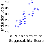
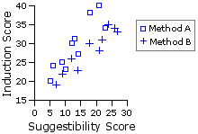
X = the score on the index of primary suggestibility Y = the score on the index of hypnotic induction

	Method A				Method B
Sub- ject	Xa	Ya		Sub- ject	Xb	Yb
a1   a2   a3   a4   a5   a6   a7   a8   a9   a10	5 10 12   9 23 21 14 18   6 13	20 23 30 25 34 40 27 38 24 31		b1   b2   b3   b4   b5   b6   b7   b8   b9   b10	7 12 27 24 18 22 26 21 14   9	19 26 33 35 30 31 34 28 23 22
Means	13.1	29.2			18.0	28.1

If you have not already done so, please click here to place a version of the data table into the frame on the left.

---

A basic one-way analysis of covariance requires four sets of calculations. In the first set you will clearly recognize the analysis-of-variance aspect of ANCOVA. The two middle sets are aimed at the covariance aspect, and the final set ties the two aspects together. As in earlier chapters, SS refers to the sum of squared deviates. The designation SC in the third set refers to the sum of co-deviates, the raw measure of covariance introduced in Chapter 3. In both cases, the subscripts "T," "wg," and "bg" refer to "Total," "within-groups," and "between-groups," respectively.

---

1. SS values for Y, the dependent variable in which one is chiefly interested._T
   

   Items to be calculated:  SST(Y)  SSwg(Y)  SSbg(Y)

   ---

2. SS values for X, the covariate whose effects upon Y one wishes to bring under statistical control.
   

   Items to be calculated:  SST(X)  SSwg(X)

   ---

3. SC measures for the covariance of X and Y;
   

   Items to be calculated:  SCT  SCwg

   ---

4. And then a final set of calculations, which begin by removing from the Y variable the portion of its variability that is attributable to its covariance with X.

   ---

The calculations for the first two of these sets are exactly like those for a one-way independent-samples ANOVA, as described in Chapter 14. I will therefore show only the results of the calculations, along with the summary values on which they are based, and leave it to you to work out the computational details. If there is any step in these first two sets of calculations that you find unclear, it would be a good idea to go back and review Chapter 14.

---

1. Calculations for the Dependent Variable Y

The following table shows the values of Y along with the several summary statistics required for the calculation of SS_T(Y), SS_wg(Y), and SS_bg(Y):

	Ya	Yb
	20 23 30 25 34 40 27 38 24 31	19 26 33 35 30 31 34 28 23 22	for total array of data		Click here if you wish to see the details of calculation for this data set.
N	10	10	20		SST(Y) = 668.5  SSwg(Y) = 662.5  SSbg(Y) = 6.0
.∑Yi	292	281	573
.∑Yi2	8920	8165	17085
SS	393.6	268.9
Mean	29.2	28.1	28.7

Just as an aside, note the discrepancy between  SSbg(Y)=6.0 [0.9% of total variability] and  SSwg(Y)=662.5 [99.1% of total variability] This reflects the fact mentioned earlier, that the mean difference between the groups is quite small in comparison with the variability that exists inside the groups.

---

2. Calculations for the Covariate X

The next table has the same structure as the one above, but now what we show are the values of X along with the several summary statistics required for the calculation of SS_T(X) and SS_wg(X). (We need not bother with SS_bg(X), since it does not enter into any subsequent calculations.)

	Xa	Xb
	5 10 12   9 23 21 14 18   6 13	7 12 27 24 18 22 26 21 14   9	for total array of data		Click here if you wish to see the details of calculation for this data set.
N	10	10	20		SST(X) = 908.9  SSwg(X) = 788.9
.∑Xi	131	180	311
.∑Xi2	2045	3700	5745
SS	328.9	460.0
Mean	13.1	18.0	15.6

---

3. Calculations for the Covariance of X and Y

You will recall from Chapter 3 that the raw measure of the covariance between two variables, X and Y, is a quantity known as the sum of co-deviates:

	SC = ∑(Xi—MX)(Yi—MY)		(Xi—MX) = deviateX (Yi—MY) = deviateY (Xi—MX)(Yi—MY) = co-deviateXY

which for practical computational purposes can be expressed as

	SC	= ∑(XiYi) —	(∑Xi)(∑Yi) N

We will be calculating two separate values of SC: one for the covariance of X and Y within the total array of data, and another for the covariance within the two groups.

The next table shows the cross-products of X_i and Y_i for each subject in each of the two groups. (E.g., the first subject in group A had X_i=5 and Y_i=20; hence X_iY_i=100.) Also shown are the separate sums of X_i and Y_i within each group and for the total array of data, as these values will also be needed for the calculations that follow.

	Groups
	A	B		For group A:  o∑Xai = 131  o∑Yai = 292  For group B:  o∑Xbi = 180  o∑Ybi = 281  For total array:  o∑XTi = 311  o∑YTi = 573
	XaYa	XbYb
	100 230 360 225 782 840 378 684 144 403	133 312 891 840 540 682 884 588 322 198	for total array of data
Sums	4146	5390	9536
	.∑(XaiYai)	.∑(XbiYbi)	.∑(XTiYTi)

On the basis of the summary values presented in this table you can then easily calculate SC for the total array of data as

SCT

= ∑(XTiYTi) —

(∑XTi)(∑YTi) NT

SCT

= 9536 —

(311)(573) 20

= 625.9

---

The values of SC within each of the two groups can be calculated similarly as

	For Group A:
	SCwg(a)	= ∑(XaiYai) —	(∑Xai)(∑Yai) Na

SCwg(a)

= 4146 —

(131)(292) 10

= 320.8

	For Group B:
	SCwg(b)	= ∑(XbiYbi) —	(∑Xbi)(∑Ybi) Nb

SCwg(b)

= 5390 —

(180)(281) 10

= 332.0

the sum of which will then yield the within-groups covariance measure of

	SCwg	= SCwg(a) + SCwg(b)
		= 320.8 + 332.0 = 652.8

---

4. The Final Set of Calculations

We begin with a summary of the values of SS and SC obtained so far, as these will be needed in the calculations that follow. Recall that Y is the variable in which we are chiefly interested, and X is the covariate whose effects we are seeking to remove.

	X		Y		Covariance
	SST(X) = 908.9 SSwg(X) = 788.9		SST(Y) = 668.5 SSwg(Y) = 662.5 SSbg(Y) = 6.0		SCT = 625.9 SCwg = 652.8
	For handy reference, click here to place a version of this table into the frame on the left.]

---

4a. Adjustment of SS_T(Y)

From Chapter 3 you know that the overall correlation between X and Y (both groups combined) can be calculated as

	rT	=	SCT sqrt[SST(X) x SST(Y)]
		=	625.9 sqrt[908.9 x 668.5]
		=	+.803

The proportion of the total variability of Y attributable to its covariance with X is accordingly

(rT)2 = (+.803)2 = .645

In the first step of this series, we adjust SS_T(Y) by removing from it this proportion of covariance. Given SS_T(Y)=668.5, the amount to be removed is

668.5 x .645 = 431.2

and the adjusted value of SS_T(Y) is therefore

668.5—431.2 = 237.3  [tentative]

I have marked the above result as tentative because a calculation based on r² is likely to produce rounding errors [in the present example, the 0.645 value used for (r_T)² is rounded from 0.64475...]. For practical purposes, one is better advised to use the following algebraically equivalent computational formula:

	[adj]SST(Y)	= SST(Y)—	(SCT)2 SST(X)		"[adj]" = "adjusted"
		= 668.5 —	(625.9)2 908.9
		= 237.5

---

4b. Adjustment of SS_wg(Y)

By analogy, the aggregate correlation between X and Y within the two groups can be calculated as

	rwg	=	SCwg sqrt[SSwg(X) x SSwg(Y)]
		=	652.8 sqrt[788.9 x 662.5]
		=	+.903

The proportion of the within-groups variability of Y attributable to covariance with X is therefore

(rwg)2 = (+.903)2 = .815

The amount of SS_wg(Y)(=662.5) to be removed is accordingly

662.5 x .815 = 539.9

and the adjusted value of SS_wg(Y) is therefore

662.5—539.9 = 122.6  [tentative]

Here again the result is marked tentative on account of the possibility of rounding errors. The more precise result is given by the following computational formula:

	[adj]SSwg(Y)	= SSwg(Y)—	(SCwg)2 SSwg(X)
		= 662.5 —	(652.8)2 788.9
		= 122.3

---

4c. Adjustment of SS_bg(Y)

The adjusted value of SS_bg(Y) can then be obtained through simple subtraction as

	[adj]SSbg(Y)	=	[adj]SST(Y) — [adj]SSwg(Y)
		=	237.5 — 122.3 = 115.2

---

4d. Adjustment of the Means of Y for Groups A and B

A moment ago, while adjusting the value of SS_wg(Y), we spoke of the aggregate correlation between X and Y within the two groups. Although this particular correlation is rather more abstract than the correlations one normally encounters, it is nonetheless a genuine correlation; and, as such, it can be described by a regression line defined by its slope and intercept. Our immediate interest is in its slope, which on analogy with the concept of slope presented in Chapter 3 can be calculated as

	bwg	=	SCwg SSwg(X)
		=	652.8 788.9	= +.83

Recall that the slope of the regression line is the measure of the average amount by which Y increases or decreases as a function of X. In the present example, an increase by 1 unit of X is associated with an average increase of .83 units of Y; an increase by 2 units of X is associated with an average increase of 2x.83=1.66 units of Y; and so forth. Similarly, a decrease by 1 unit of X is associated with an average decrease of .83 units of Y; a decrease by 2 units of X is associated with an average decrease of 2x.83=1.66 units of Y; and so on.

And now for our what-if scenario. Suppose that both groups had started out with the same mean level of suggestibility: namely, 15.55, which is the mean of X for both groups combined. In this case, group A would have been starting out with a mean suggestibility level 2.45 units higher than it actually started with, while group B would have been starting out with a mean suggestibility level 2.45 units lower. Given the observed dependence of Y on X, the respective means of the two groups would therefore presumably have been on the order of

	[adj]MYa = 29.2 + (2.45x.83) = 31.23
and
	[adj]MYb = 28.1 — (2.45x.83) = 26.07

This is the conceptual structure for the adjustment of the means of Y for the groups. Once you have the concept, the mechanics of the process can be accomplished somewhat more expeditiously via the following computational formula:

	For Group A:
	[adj]MYa	= MYa — bwg(MXa—MXT)
		= 29.2 — .83(13.1—15.55)
		= 31.23

	For Group B:
	[adj]MYb	= MYb — bwg(MXb—MXT)
		= 28.1 — .83(18.0—15.55)
		= 26.07

---

4e. Analysis of Covariance Using Adjusted Values of SS

As with the corresponding one-way ANOVA, the final step in a one-way analysis of covariance involves the calculation of an F-ratio of the general form

F =

MSeffect MSerror

=

MSbg MSwg

=

SSbg/dfbg SSwg/dfwg

The only difference is that now we are using the adjusted values of SS_bg(Y) and SS_wg(Y), along with one adjusted value of df. In the basic analysis of variance, the degrees of freedom for the within-groups variance is N_T—k, where k is the number of groups and N_T is the total number of subjects. In the analysis of covariance the number of within-groups degrees of freedom is reduced by one to accommodate the fact that the covariance portion of within-groups variability has been removed from the analysis. Hence the adjusted value of df_wg(Y) is

[adj]dfwg(Y) = NT—k—1

for the present example:   20—2—1 = 17

The degrees of freedom for the between-groups condition remains the same as for the one-way ANOVA:

dfbg(Y) = k—1

for the present example:   2—1 = 1

Given [adj]SS_bg(Y)=115.2 and [adj]SS_wg(Y)=122.3, our F-ratio for the analysis of covariance is accordingly

	F	=	[adj]SSbg(Y)/dfbg(Y) [adj]SSwg(Y)/[adj]dfwg(Y)
		=	115.2/1 122.3/17
		=	16.01 [with df=1,17]

As you can see from the adjacent portion of Appendix D, our calculated value of F=16.01 is significant well beyond the .01 level for df=1,17. Please note carefully, however, that the interpretation of a significant F-ratio in an analysis of covariance is a bit trickier than it would be if this were just a plain, garden-variety ANOVA. It does not entail that the difference between the originally observed means of the two samples,

	MYa=29.2  versus  MYb=28.1

is significant in and of itself. The claim it is making is a somewhat more complex one, tied together by several logical constructions of the if/then variety:

• If the correlation between X and Y within the general population is approximately the same as we have observed within the samples; and_T
  
• If we remove from Y the covariance that it has with X, so as to remove from the analysis the pre-existing individual differences that are measured by the covariate X; and_T
  
• If we adjust the group means of Y in accordance with the observed correlation between X and Y;_T
  
• Then we can conclude that the two adjusted means

  	[adj]MYa=31.23  versus  [adj]MYb=26.07

  significantly differ in the degree indicated, namely, P<.01, and thus that Method A is more effective than Method B.

This, however, does not distinguish the analysis of covariance fundamentally from ANOVA or any other inferential statistical procedure, for they are all wrapped up in a chain of if/then logical constructions. It is simply that the chain for the analysis of covariance is a few links longer.

---

¶Assumptions of ANCOVA

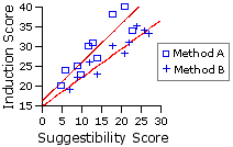
The analysis of covariance has the same underlying assumptions as its parent, the analysis of variance. It also has the same robustness with respect to the non-satisfaction of these assumptions, providing that all groups have the same number of subjects. There is, however, one assumption that the analysis of covariance has in addition, by virtue of its co-descent from correlation and regression—namely, that the slopes of the regression lines for each of the groups considered separately are all approximately the same.

The operative word here is "approximately." Because of random variability, it would rarely happen that two or more samples of bivariate XY values would all end up with precisely the same slope, even though the samples might be drawn from the very same population. And so it is for the slopes of the separate regression lines for our two present samples. They are clearly not precisely the same. The question is, are they close enough to be regarded as reflecting the same underlying relationship between X and Y? In the calculations of step 4d, we found the slope of the line for the overall within-groups regression to be b_wg=+.83, and that was the value used in adjusting the means of group A and group B. The analysis of covariance is assuming that the slopes of the separate regression lines for the two samples do not significantly differ from +.83. We will examine this assumption more thoroughly in Part 3, after working through our second computational example.