©Richard Lowry, 1999-
All rights reserved.
Chapter 8.
Chi-Square Procedures for the Analysis of Categorical
Part 3
Chi-square procedures for two dimensions of categorization are not limited to the case where there are just two rows and two columns. In principle, they can be applied to contingency tables involving any number of rows and columns, although in practice you will not often find more than three or four of each. We will illustrate this type of application with an example involving two rows and three columns.
A team of clinical researchers is interested in assessing the effectiveness of a certain newly developed form of behavior therapy for the treatment of chronic anxiety conditions. To this end, they collect a sample of 150 persons who, although diagnosed with chronic anxiety, are currently receiving no treatment for their condition. Of these subjects, 60 are randomly selected to receive a two-month program of the behavior therapy, while the remaining 90 continue to receive no treatment. At the end of the two-month period, all 150 subjects are assessed with respect to whether their anxiety condition has improved, grown worse, or remained essentially unchanged. The following contingency table shows the results of this study, cross-categorized according to the two variables (i) therapy vs. no therapy and (ii) improved, worse, or no change (N/C). Also shown here, in parentheses, are the percentage figures within each of the two rows.
And here is a graph of the outcome, portrayed in terms of the percentages of subjects within each of the two groups who ended up being assessed as improved, worse, or no change.
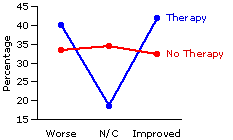
So the investigators do appear to have found a difference between the two groups, though it is not the simple difference they might have expected. Sure enough, the percentage of those assessed as "improved" is greater within the therapy group than within the no-therapy group (41.7% vs. 32.2%); but at the same time, the percentage judged "worse" within the therapy group is also greater (40.0% vs. 33.3%). Might it be that this particular form of therapy has positive effects for some chronic-anxiety subjects and negative effects for others? If so, the researchers would certainly want to investigate further, to determine just what spells the difference between those cases where the effects are positive and those where they are negative.
But of course there is no point in doing anything at all until it can be established that the observed difference between the therapy and no-therapy groups reflects anything other than mere chance coincidence. The first of the following two tables shows the calculations for expected cell frequencies and the second details the calculations for the cell components of chi-square.
Thus:
With two rows and three columns, degrees of freedom is equal to 2, so that is the sampling distribution of chi-square to which this value gets referred. Figure 8.7 shows the shape of the sampling distribution fordf=2, along with the values of chi-square required for several levels of significance.
Figure 8.7. Sampling Distribution of Chi Square for df=2.
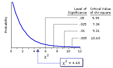
As you can see, the calculated value of =4.68
=4.68So our investigators, unable to reject the null hypothesis, cannot confidently conclude anything at all about the effects of this form of therapy, one way or the other. All that work for nothing!
Ah! But suppose, as shown below, that they had started out with samples twice the size and ended up with the same proportionate results.
Exactly the same proportions. Exactly the same graph.

But now (I will leave the computational details to you) they would end up with =9.35,
Figure 8.8. Sampling Distribution of Chi Square for df=2.
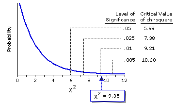
In this second scenario the researchers could reject the null hypothesis with a high degree of confidence, and could accordingly infer that the therapy does have the effect suggested by the observed differences between the therapy and no-therapy groups. At the beginning of Chapter 5, while laying out some basic concepts of probability, we noted that the mere-chance likelihood of getting as many as 70% heads in N tosses of a coin is fairly large (.17) when N=10 and very tiny (.00005) when N=100. It is the same principle at work here in these two chi-square scenarios. For any particular proportionate difference between an observed value and the corresponding mean chance expected value: the larger the sample, the less likely it is that a difference that large or larger will occur by mere chance coincidence; hence the greater will be the statistical significance of such a difference.
Avoiding an Egregious Logical Fallacy: Interlude on What NOT to do with a Non-Significant Chi-Square Value
There is an important implication here that we must take a moment to draw out. By way of analogy, suppose you were planning to hike through a forest; but before you hike very far, you want to determine whether the forest includes among its denizens a certain species of large, irritable bear. So you cautiously sample a limited area of the forest to see whether there are any signs of the bear. Your null hypothesis is that the bear is not present in the forest. And here are the two possible outcomes of your investigation: Either you find indications of the bear's presence—its growlings, droppings, perhaps even a visual sighting—or you do not. In the first case, you could reject the null hypothesis with a certain degree of confidence and conclude that the bear probably does abide there, in which event you might wish to choose a different venue for your hike. This much is fairly obvious. But what can you you conclude in the second case, when the outcome is negative? You have looked for the bear and found no sign of it. Does that permit you to conclude that the species is probably not to be found in the forest?
The short answer is that this second outcome would allow you to conclude nothing at all with any degree of confidence. Of course, it might be that the bear truly is absent from the forest. But then again, it might be that you have simply not sampled enough of the forest. There is a certain tendency of the human mind to assume that if we look for something and do not find it, then it does not exist. It is a fundamental error of logic, obviously to be avoided in the case of irritable bears, and no less to be eschewed with tests of statistical significance.
There is a certain application of the chi-square procedures for a one-dimensional situation, known as the chi-square goodness-of-fit test, that rests in my view on this same basic logical fallacy. The following example is rather fanciful, but not at all far-fetched.
Suppose a researcher frames the hypothesis that four variations on a certain genetic characteristic, A, B, C, and D, exist within the muglout species in the proportions:A=20%, B=30%, C=30%, and D=20%. To test his hypothesis, he examines N=60 randomly selected muglouts and sorts each according to whether it displays variation A, B, C, or D. The following table shows the results he obtained (O), laid out in comparison with the results that would have been predicted (E) on the basis of his genetic hypothesis.
Performing the requisite calculations, our investigator finds a non-signigicant chi-square valueof 2.5 (for df=3 a value of 7.81 would be required for significance at the minimal .05 level) and joyfully exclaims: "Aha! Although the observed pattern of frequencies does differ a bit from the pattern stipulated by my hypothesis, it does not differ significantly. Therefore—it's a fit! My hypothesis is supported by the data. Tenure Heaven, here I come!"
The logical fallacy in this scenario is contained in the phrase "Therefore—it's a fit!" The non-significant test result in this case would allow the investigator to conclude that this particular sample provides no evidence contradicting his hypothesis. But the absence of evidence contradicting an hypothesis is not at all the same thing as positive evidence in support of an hypothesis. Indeed, the pattern of frequencies and percentages observed in this particular sample would be consistent with (would not significantly differ from the pattern stipulated by) any number of other hypotheses that the investigator might have framed. The pattern predicted by the investigator's hypothesis was
[E1] A=20%, B=30%, C=30%, D=20%.
Suppose that he had instead predicted quite the opposite:
[E2] A=30%, B=20%, C=20%, D=30%.
Similarly, if the same proportionate outcome had been found in a sample ofN=200 muglouts,
the resulting chi-square valueof 8.33 would be significant beyond the .05 level, and our investigator's ascension to Tenure Heaven would accordingly have to be postponed.
The principle at stake here is one that applies not just to chi-square, but to statistical tests in general. It is that, while a significant test result permits you to reject the null hypothesis with a certain degree of confidence, a non-significant result does not allow you to accept the null hypothesis.
Two Limitations on the Use of Chi-Square Procedures
Although chi-square procedures are computationally simple, they rest upon a rather complex logical substructure; and this, in turn, imposes certain limitations on how they can be applied. Two of these in particular are worth mentioning at the present time.
End of Chapter 8, Part 3.
Return to Top of Chapter 8, Part 3
Go to Chapter 8a [The Fisher Exact Probability Test]
Go to Chapter 9 [Introduction to Procedures Involving Sample Means]
A team of clinical researchers is interested in assessing the effectiveness of a certain newly developed form of behavior therapy for the treatment of chronic anxiety conditions. To this end, they collect a sample of 150 persons who, although diagnosed with chronic anxiety, are currently receiving no treatment for their condition. Of these subjects, 60 are randomly selected to receive a two-month program of the behavior therapy, while the remaining 90 continue to receive no treatment. At the end of the two-month period, all 150 subjects are assessed with respect to whether their anxiety condition has improved, grown worse, or remained essentially unchanged. The following contingency table shows the results of this study, cross-categorized according to the two variables (i) therapy vs. no therapy and (ii) improved, worse, or no change (N/C). Also shown here, in parentheses, are the percentage figures within each of the two rows.
| Worse | N/C | Improved|
| Therapy | 24 | (40.0%) 11 | (18.3%) 25 | (41.7%) 60 | No Therapy | 30 | (33.3%) 31 | (34.4%) 29 | (32.2%) 90 |
| 54 | 42 | 54 | 150 | | |||
And here is a graph of the outcome, portrayed in terms of the percentages of subjects within each of the two groups who ended up being assessed as improved, worse, or no change.

So the investigators do appear to have found a difference between the two groups, though it is not the simple difference they might have expected. Sure enough, the percentage of those assessed as "improved" is greater within the therapy group than within the no-therapy group (41.7% vs. 32.2%); but at the same time, the percentage judged "worse" within the therapy group is also greater (40.0% vs. 33.3%). Might it be that this particular form of therapy has positive effects for some chronic-anxiety subjects and negative effects for others? If so, the researchers would certainly want to investigate further, to determine just what spells the difference between those cases where the effects are positive and those where they are negative.
But of course there is no point in doing anything at all until it can be established that the observed difference between the therapy and no-therapy groups reflects anything other than mere chance coincidence. The first of the following two tables shows the calculations for expected cell frequencies and the second details the calculations for the cell components of chi-square.
Expected Cell Frequencies|
| Worse | N/C | Improved |
| Therapy | 60x54 | 150 = 21.6 60x42 | 150 = 16.8 60x54 | 150 = 21.6 60 | No | Therapy 90x54 | 150 = 32.4 90x42 | 150 = 25.2 90x54 | 150 = 32.4 90 |
| 54 | 42 | 54 | 150 | | |||||||
Recall that the calculation of chi-square requires a correction for continuity only when there are exactly two rows and two columns.
| (O—E)2 E |
Thus:
Cell Components of Chi-Square|
| Worse | N/C | Improved |
| Therapy |
(24—21.6)2 | 21.6 = 0.27
(11—16.8)2 | 16.8 = 2.00
(25—21.6)2 | 21.6 = 0.54
| No | Therapy
(30—32.4)2 | 32.4 = 0.18
(31—25.2)2 | 25.2 = 1.33
(29—32.4)2 | 32.4 = 0.36
|
| sum: | | ||||||||||
With two rows and three columns, degrees of freedom is equal to 2, so that is the sampling distribution of chi-square to which this value gets referred. Figure 8.7 shows the shape of the sampling distribution for
Figure 8.7. Sampling Distribution of Chi Square for df=2.

As you can see, the calculated value of
Ah! But suppose, as shown below, that they had started out with samples twice the size and ended up with the same proportionate results.
| Worse | N/C | Improved|
| Therapy | 48 | (40.0%) 22 | (18.3%) 50 | (41.7%) 120 | No Therapy | 60 | (33.3%) 62 | (34.4%) 58 | (32.2%) 180 |
| 108 | 84 | 108 | 300 | | |||
Exactly the same proportions. Exactly the same graph.

But now (I will leave the computational details to you) they would end up with
Figure 8.8. Sampling Distribution of Chi Square for df=2.

In this second scenario the researchers could reject the null hypothesis with a high degree of confidence, and could accordingly infer that the therapy does have the effect suggested by the observed differences between the therapy and no-therapy groups. At the beginning of Chapter 5, while laying out some basic concepts of probability, we noted that the mere-chance likelihood of getting as many as 70% heads in N tosses of a coin is fairly large (.17) when N=10 and very tiny (.00005) when N=100. It is the same principle at work here in these two chi-square scenarios. For any particular proportionate difference between an observed value and the corresponding mean chance expected value: the larger the sample, the less likely it is that a difference that large or larger will occur by mere chance coincidence; hence the greater will be the statistical significance of such a difference.
Avoiding an Egregious Logical Fallacy: Interlude on What NOT to do with a Non-Significant Chi-Square Value
There is an important implication here that we must take a moment to draw out. By way of analogy, suppose you were planning to hike through a forest; but before you hike very far, you want to determine whether the forest includes among its denizens a certain species of large, irritable bear. So you cautiously sample a limited area of the forest to see whether there are any signs of the bear. Your null hypothesis is that the bear is not present in the forest. And here are the two possible outcomes of your investigation: Either you find indications of the bear's presence—its growlings, droppings, perhaps even a visual sighting—or you do not. In the first case, you could reject the null hypothesis with a certain degree of confidence and conclude that the bear probably does abide there, in which event you might wish to choose a different venue for your hike. This much is fairly obvious. But what can you you conclude in the second case, when the outcome is negative? You have looked for the bear and found no sign of it. Does that permit you to conclude that the species is probably not to be found in the forest?
The short answer is that this second outcome would allow you to conclude nothing at all with any degree of confidence. Of course, it might be that the bear truly is absent from the forest. But then again, it might be that you have simply not sampled enough of the forest. There is a certain tendency of the human mind to assume that if we look for something and do not find it, then it does not exist. It is a fundamental error of logic, obviously to be avoided in the case of irritable bears, and no less to be eschewed with tests of statistical significance.
There is a certain application of the chi-square procedures for a one-dimensional situation, known as the chi-square goodness-of-fit test, that rests in my view on this same basic logical fallacy. The following example is rather fanciful, but not at all far-fetched.
Suppose a researcher frames the hypothesis that four variations on a certain genetic characteristic, A, B, C, and D, exist within the muglout species in the proportions:
| A | B | C | D | Totals | 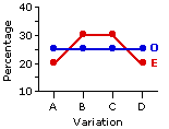
| |||||||||||
| O | 15 (25.0%) | 15 (25.0%) | 15 (25.0%) | 15 (25.0%) | 60| E | 12 | (20.0%) 18 | (30.0%) 18 | (30.0%) 12 | (20.0%) 60 |
| | ||||
Performing the requisite calculations, our investigator finds a non-signigicant chi-square value
The logical fallacy in this scenario is contained in the phrase "Therefore—it's a fit!" The non-significant test result in this case would allow the investigator to conclude that this particular sample provides no evidence contradicting his hypothesis. But the absence of evidence contradicting an hypothesis is not at all the same thing as positive evidence in support of an hypothesis. Indeed, the pattern of frequencies and percentages observed in this particular sample would be consistent with (would not significantly differ from the pattern stipulated by) any number of other hypotheses that the investigator might have framed. The pattern predicted by the investigator's hypothesis was
Suppose that he had instead predicted quite the opposite:
| As suggested by the adjacent graph, this mirror-image null hypothesis would have yielded precisely the same non-significant chi-square value | 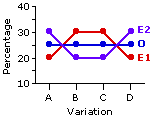
|
Similarly, if the same proportionate outcome had been found in a sample of
| A | B | C | D | Totals | 
| |||||||||||
| O | 50 (25.0%) | 50 (25.0%) | 50 (25.0%) | 50 (25.0%) | 200| E | 40 | (20.0%) 60 | (30.0%) 60 | (30.0%) 40 | (20.0%) 200 |
| | ||||
the resulting chi-square value
The principle at stake here is one that applies not just to chi-square, but to statistical tests in general. It is that, while a significant test result permits you to reject the null hypothesis with a certain degree of confidence, a non-significant result does not allow you to accept the null hypothesis.
Two Limitations on the Use of Chi-Square Procedures
Although chi-square procedures are computationally simple, they rest upon a rather complex logical substructure; and this, in turn, imposes certain limitations on how they can be applied. Two of these in particular are worth mentioning at the present time.
Restriction 1. Chi-square procedures can be legitimately applied only if the categories into which the N observations are sorted are independent of each other; that is, only if the placement of each observation into a particular category does not in any way depend on the placement of any of the other observations. For the beginning student of the subject, this restriction is best observed by ensuring that the categories are both exhaustive and mutually exclusive, such that each observation fits into one or another of the categories and no observation fits into more than one. Restriction 2. The logical validity of the chi-square test is greatest when the values of E, the mean chance expected frequencies within the cells, are fairly large, and decreases as these values of E become smaller. Although the statistical cognoscenti do not always agree on just where to draw the line between "large enough" and "too small," the beginning student can take this as a practical rule of thumb: Chi-square procedures can be legitimately applied only if all values of E are equal to or greater than 5. For the special case of two rows by two columns, this limitation can usually be circumvented through application of the Fisher Exact Probability Test, which you will find covered in Chapter 8a. |
|
This chapter includes an Appendix that will generate a graphic and numerical display of the properties of the sampling distribution of chi-square for any particular value of degrees of freedom, up through |
End of Chapter 8, Part 3.
Return to Top of Chapter 8, Part 3
Go to Chapter 8a [The Fisher Exact Probability Test]
Go to Chapter 9 [Introduction to Procedures Involving Sample Means]
| Home | Click this link only if the present page does not appear in a frameset headed by the logo Concepts and Applications of Inferential Statistics |