©Richard Lowry, 1999-
All rights reserved.
Chapter 8.
Chi-Square Procedures for the Analysis of Categorical
Part 1
The binomial procedures described in Chapters 5 and 6 apply to situations where there are exactly two mutually exclusive categories into which observations might fall—female/male, head/tail, recovery/non-recovery, and so on. The family of inferential statistical procedures known as chi-square (pronounced 'kai' to rhyme with 'sky') extends the logic of binomial procedures to cover situations where there are more than two categories of possible outcome; for example, students categorized according to academic class (freshman, sophomore, junior, senior) or patients with a certain disease categorized according to whether their condition, following an experimental treatment, is improved, worsened, or unchanged. Chi-square procedures also extend this logic to cover situations where there is more than one dimension of classification; for example, students categorized according to whether they describe themselves as "conservative" or "liberal," as well as by their academic class as freshman, sophomore, junior, or senior. When the observed items—students or whatever else they might be—are categorized in this fashion according to two or more separate dimensions of classification concurrently, they are said to be cross-categorized. We will begin with the simpler situation in which there is only one dimension of categorization.
Chi-Square Procedures for One Dimension of Categorization
The underlying logic of chi-square would be best illustrated with the example of tossing a three-sided coin, with each of the sides having an outcome probability of exactly one-third. But as a coin with these specifications is difficult to imagine, we will have to improvise with an analogy.
For more than a century, the three species of large fish—gumpies, sticklebarbs, and spotheads—that are native to a certain river have been observed to co-exist in equal proportions of one-third each. But now a random sample of 300 large fish drawn from a standard fish-sampling location has turned up numbers and proportions suggesting that something has occurred to upset the natural ecology of the river. If the three fish species still inhabited the river in equal proportions, we would expect to find about 100 instances of each in a sample of size N=300; whereas what we actually observe are 89 gumpies, 120 sticklebarbs, and 91 spotheads. Here is an overview of the observed counts and percentages for the three fish-species categories, each in comparison with the corresponding mean chance expected values (MCE).
The question of statistical significance in this situation is of the same form we have already encountered, except that here what is at issue is the difference between two patterns, namely, the observed frequency pattern of89/120/91 versus the MCE frequency pattern of 100/100/100. And the first step in answering the question is to devise a way for measuring the degree to which the two patterns differ from each other in the aggregate. A straightforward way of going about this would be to take, for each of the three categories, the difference between the observed frequency and the expected frequency, and then divide that difference by the expected frequency.
The outcome of this operation would be a measure of the proportionate amount by which each observed frequency deviates from its corresponding expected frequency. Thus
In percentage terms, the observed number of gumpies in the sample is 11 percent smaller than the corresponding MCE frequency, the number of sticklebarbs is 20 percent greater, and the number of spotheads is 9 percent smaller.
The advantage of this procedure is that you will find it intuitively obvious just what is being measured. Its limitation is that the proportionate differences measured for the several categories—in the present example, —.11, +.20, and —.09—will always sum to zero and thus will not be able to provide a measure of how much the observed and expected patterns of frequencies differ from each other overall. The simple way to surmount this limitation is the same as we examined in Chapter 2 when we spoke of deviates and squared deviates in connection with measures of variability. That is, instead of taking just the difference between an observed frequency and its corresponding expected frequency, we take the squared difference.
The effect of this operation will be to get rid of the minus signs and thus provide a set of measures whose sum will reflect the aggregate degree of difference that actually exists between the observed and expected patterns of frequencies. For the present example, where the patterns are 89/120/91 and 100/100/100, it comes out as
This, in brief, is the measure known as chi-square, conventionally rendered in symbolic notationas  ,
, which is simply the lower-case Greek letter 'chi' ('kai') with a squaring sign appended. For the sake of simplicity, we will henceforth represent an observed frequency as O and its corresponding MCE expected frequency as E. The only other item of symbolic notation is the summation sign,  ,
, with which you are already familiar. Henceforth we will also be describing each category (e.g., gumpies, sticklebarbs, spotheads) as a cell; this is merely a linguistic convention reflecting the box-like tabular format usually employed for representing categorical frequency data within the context of chi-square procedures.
Here, then, is the simple two-step operation for calculating for the general case where there is one dimension of categorization. Keep in mind that what we are measuring through this procedure is the degree to which an observed pattern of frequencies differs, overall, from an MCE expected pattern.
First, for each cell, calculate the component value
which, as we have just seen, yields
and then: sum up these several component values to get the overall value of chi-square, according to the formulaT
If we were building the inferential apparatus of chi-square from scratch, our next task would be to figure out the properties of the sampling distribution to which this or any other calculated value of belongs. Fortunately, that particular wheel has already been invented, and we do not need to try to reinvent it. For the sake of illustration, however, suppose for just a moment that we were starting from scratch and had no idea at all of the sampling distribution to which our calculated value of
  =6.02
=6.02
Until fairly recently it would have required a quite high level of mathematical expertise and acumen to figure out the answer to this question from scratch. The only alternative method would have been to construct the sampling distribution of chi-square empirically. That is, start out with a river that you know in advance contains vast numbers of gumpies, sticklebarbs, and spotheads in exactly equal proportions of one-third each; draw a random sample of size N=300; calculate and record the resulting value of chi-square—and then repeat that operation again and again, many times over. After a very large number of such samples, we would then take the proportion of cases in which the calculated chi-square value was equal to or greater than 6.02—and that would be our probability value, or at least a quite close estimate of it.
The limitations of this empirical method will surely be obvious. First we would have to find a river with those precise specifications; and then we would have to devote quite a lot of time, energy, and expense to the task of drawing a multitude of samples from it. Until quite recently it would have been difficult if not impossible to construct sampling distributions in this fashion. Nowadays, on the other hand, it can be done quite easily—or at least simulated—within the virtual reality of a computer. Using a programmable spreadsheet application, I instructed the desktop computer in my office to perform exactly the empirical sampling procedure just described—the only material difference being that what the computer was pulling up in its nets was not random gumpies, sticklebarbs, and spotheads, but random a's, b's, and c's. The programming instructions were of course given in a language the computer understands. Here is the English translation:
Figure 8.1 shows the distribution of the 10,000 chi-square values that resulted from this simulation. The format of the graph is that of a histogram, with relative frequencies expressed in terms of percentages. Thus, the first column on the left represents the percentage of chi-square values that fell between zero and .99; the second column shows the percentage that fell between 1.0 and 1.99; and so on. As indicated on the right-hand side of the graph, the 10,000 sample values of chi-square included only 4.99 percent that were equal to or greater than our originally calculated valueof  =6.02—
 from which we would infer that the mere chance probability of the outcome observed in our fish example is somewhere in the vicinity of P=.0499.
Figure 8.1. Empirical Approximation of a Chi-Square Sampling Distribution
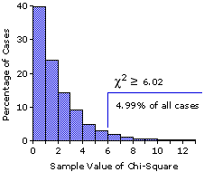
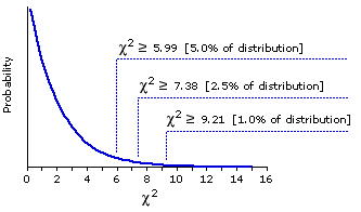
Figure 8.2 shows the "official" abstract theoretical sampling distribution of chi-square that would apply to our fish example, and you will certainly see that the correspondence between the two is very close. In the theoretical distribution, the critical value of chi-square for significance at the P=.05 level is =5.99.
 =6.02
=6.02of  =6.02.
 Figure 8.2 also shows the critical values of chi-square for significance at the .025 (2.5 percent) and .01 (1.0 percent) levels.
Figure 8.2. Theoretical Sampling Distribution of Chi-Square (df=2)
Although this next point will be obvious from the way in which chi-square values are calculated—with the difference between O and E squared to get rid of the minus signs—do take a moment nonetheless to notice that there are no negative chi-square values. All possible valuesof 
in this or any other chi-square sampling distribution are either equal to or greater than zero. The immediate implication of this fact is that a chi-square test of statistical significance is intrinsically non-directional. In our fish example there are several possible directions in which the results might have gone. What we in fact ended up with was more observed sticklebarbs than expected and fewer gumpies and spotheads:
But we might also have ended up with a preponderance of gumpies or spotheads; or alternatively, with a preponderance of any two of the species along with relatively small numbers of the third. Any one of these possibilities, providing it involved a sufficiently large discrepancy between the patterns of O and E, would have resulted in a chi-square value equal or greater than the valueof  =6.02
=6.02 calculated for our example. The following two possibilities, among others, would each have resulted in chi-square values exactly equal to 6.02.
We will see later that there are certain circumstances in which the apparatus of chi-square can be adjusted to provide a directional test of significance; but until then, the basic precept is that a chi-square test of statistical significance is intrinsically non-directional.
The essential difference between the graphs inFigures 8.1 and 8.2 is not that one is a histogram and the other is a smoothed polygon. It is rather that one is fairly specific and the other broadly general. Strictly speaking, the simulated sampling distribution shown in Figure 8.1 applies only to situations that correspond to the stipulated details of the simulation; namely, that there are three categories, the size of the sample is N=300, and the pattern of MCE frequencies for the three categories is 100/100/100. The theoretical distribution of Figure 8.2, on the other hand, includes cases of this particular type, but also extends more generally beyond them to all other three-category situations, irrespective of the size of the sample or the particular values of the expected frequencies; for example, a sample of size N=100 with expected frequencies of 25/50/25, or of size N=62 with expected frequencies of 13/22/27.
If our sample of fish had been sorted into four categories, or five, or six, on the other hand, we would need to refer to a different member of the family of chi-square sampling distributions. So long as we are dealing with only one dimension of categorization, the sampling distribution of chi-square that is appropriate for any particular case is determined quite simply by the number of categories—3, 4, 5, 9, 12, or whatever it might be. With two or more dimensions of categorization it becomes a bit more complex, as you will see later in this chapter. In both kinds of cases, the appropriate sampling distribution of chi-square is determined not by the number of categories as such, but rather by a more general property spoken of as degrees of freedom, symbolized as df. In working to understand the meaning of this concept, your first step should be to disentangle it entirely from most of the meanings that you normally associate with the word "freedom," since in this context it has nothing at all to do with freedom of the will, freedom of conscience, or anything of the sort. Degrees of freedom, df, is simply an index of the amount of random variability, mere chance coincidence, that can be present in a particular situation. Its closest literal translation would be something along the line of "degrees of arbitrariness."
Here is a working definition of the concept that should prove sufficient for our immediate purposes. Suppose you have two cells such as the ones shown below, and you are free to plug any integer numbers that you want into them, subject only to the stipulation that the sum of the two numbers must be equal to a certain specified quantity. For purposes of illustration we will set the sum at 20, though it could actually be any positive integer value.
It will be obvious at a glance that your "freedom" in this case is limited by the fixed sum of 20. If you start by plugging the integer 8 into cell a, the number that goes into b is then inescapably fixed as20—8=12. Start by plugging 16 into cell b and the number that goes into a is then rigidly fixed as 20—16=4. So in this two-cell situation, only one of the cells is "free" to vary arbitrarily—which is to say, there is only one degree of freedom. If you have three cells subject to a fixed sum of 20
you can plug numbers arbitrarily into any two of the cells, but once those cells are plugged the value of the third is rigidly fixed. Thus, plug 6 into any one cell and 8 into either of the remaining two, and the value of the third is then fixed as20—6—8=6. So here, with three cells, your degrees of freedom would be equal to two. The same logic then extends to cases where the number of cells is four, five, six, and so on. When applying chi-square procedures to situations in which there is only one dimension of categorization, the general principle for determining degrees of freedom is
df = (number of cells)—1
In our fish example the number of categorical cells is three; hence df=2. Similarly, the chi-square sampling distribution shown in Figure 8.2 applies to the general case where df=2.
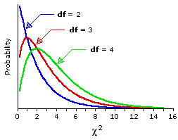
Figure 8.3 shows the same df=2 sampling distribution that appears in Figure 8.2, along with two other members of the family of chi-square sampling distributions, the ones for df=3 and df=4. We need not be distracted just now by the fact that these three distributions have somewhat different shapes on the left-hand side of the scale. What is of immediate relevance are the similarities and differences that appear on the right-hand side of the scale, in the tails of the distributions. The similarity among all three distributions is that values of chi-square in the tail regions become less probable, hence more significant, as they increase in size. And the difference is that the mere chance probability of any particular value of chi-square is greater for a larger value of df than for a smaller value. Thus, for all three distributions a value falling at or beyond =6
=6 =5;
=5;for df=2. This point will be most readily visible if you draw a vertical line in Figure 8.3 straight up from the point on the scale at which  =6.0.
=6.0.
Figure 8.3. Chi-Square Sampling Distributions for df=2, 3, and 4
In the practical application of chi-square procedures, you of course do not need to examine every detail of the relevant sampling distribution; it will be sufficient just to know the critical value that a calculated value of chi-square must equal or exceed in order to be judged statistically significant. A full set of such critical values is listed in Appendix B, and a somewhat abbreviated version of the same set is shown here in Table 8.1. For the moment we will confine our attention to Table 8.1. The first column on the left in this table, labeled df, lists various values of degrees of freedom; the row across the top lists various levels of significance (P=.05, .025, etc.); and each of the other entries indicates the critical value of chi-square that an observed value must meet or exceed in order to be judged significant at a given level of significance for a given value of df. Thus, for df=2 the minimum value of chi-square required for significance at the basic P=.05 level is 5.99; for df=3 it is 7.81; for df=4 it is 9.49; and so on. For the more stringent significance level of P=.025, the required value of chi-square is 7.38 for df=2; 9.35 for df=3; 11.14 for df=4; and so on. In applying chi-square and other statistical procedures, it is conventional to speak of a given result as being either non-significant, or significant at a certain level, or significant beyond a certain level. The illustration at the bottom of Table 8.1 will give you an idea of what these three phrases mean and how they are used.
Table 8.1. Partial Table of Critical Values of Chi-Square
Each entry indicates the critical value that an observed value of chi-square must meet or exceed in order to be judged significant at a given level of significance for a given value of df.
Here is one other example to illustrate this simpler one-dimensional version of chi-square. Suppose that a questionnaire administered to a large national sample of college students included an item aimed at measuring conservativism versus liberalism on a certain issue of social/political relevance. The item took the form of a statement, and the response categories were "strongly disagree," "moderately disagree," "undecided," "moderately agree," and "strongly agree." I will leave it to your imagination to fill in the blanks concerning what the statement was and which end of the response scale was taken to reflect "conservative" or "liberal" attitudes. Suffice it to say that the percentages of response within each category were as follows:
Professor H, upon reading the results of this survey, suspects that the students at her particular college are considerably more polarized into "conservative" and "liberal" camps, in comparison with the more general population of students studied in the national sample. To test this hypothesis, she administers the same question to a random sample of 204 students at her college and then compares the pattern of responses to the pattern of the national sample.
The null hypothesis in this situation is that the responses of Professor H's 204 respondents should not differ significantly from the pattern of the national survey. Thus, the MCE expected frequency of response in the "strongly disagree" category would be 9.4% of the 204 subjects:.094x204=19.2. For the "moderately disagree" category, it would be 15.6% of the subjects: .156x204=31.8. And so on. What Professor H actually found, however, was something that seemed to fit rather well with her suspicion concerning polarization. All that remained was to determine whether the difference between the two patterns was significant. Here is an overview of the observed counts and percentages for the five response categories, each in comparison with the corresponding MCE expected values, along with the steps required for calculating chi-square.
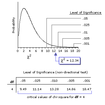
The top part of Figure 8.4 shows a graph of the sampling distribution of chi-square for the case of df=4, while the bottom part reproduces the portion of the table of critical values of chi-square that pertains to this distribution. As indicated in both the graphic and tabular parts, our observed value of =12.34
Figure 8.4. Chi-Square Sampling Distribution for df=4
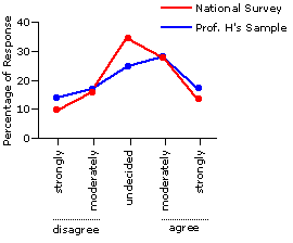
Do keep in mind, however, that the chi-square test we have just performed is intrinsically non-directional. In and of itself, the significant chi-square value says nothing at all about the particular texture or direction of the difference. Examine the details of Figure 8.5, however, and you will see that the texture of the difference is consistent with Professor H's hypothesis concerning greater conservative-liberal polarization among the students at her college. In particular, there was a smaller proportion of respondents in the "undecided" category than would have been expected on the null hypothesis, and greater proportions in the "strongly agree" and "strongly disagree" categories. These three categories, in fact, accounted for all but a small fraction of the calculated chi-square value of 12.34.
Figure 8.5. Professor H's Sample versus the Results of the National Survey
Chi-Square Procedures for One Dimension of Categorization
The underlying logic of chi-square would be best illustrated with the example of tossing a three-sided coin, with each of the sides having an outcome probability of exactly one-third. But as a coin with these specifications is difficult to imagine, we will have to improvise with an analogy.
For more than a century, the three species of large fish—gumpies, sticklebarbs, and spotheads—that are native to a certain river have been observed to co-exist in equal proportions of one-third each. But now a random sample of 300 large fish drawn from a standard fish-sampling location has turned up numbers and proportions suggesting that something has occurred to upset the natural ecology of the river. If the three fish species still inhabited the river in equal proportions, we would expect to find about 100 instances of each in a sample of size N=300; whereas what we actually observe are 89 gumpies, 120 sticklebarbs, and 91 spotheads. Here is an overview of the observed counts and percentages for the three fish-species categories, each in comparison with the corresponding mean chance expected values (MCE).
| gumpies | sticklebarbs | spotheads | Totals| Observed frequency | of cases 89 | (29.7%) 120 | (40.0%) 91 | (30.3%) 300 | Expected frequency | of cases (MCE) 100 | (33.3%) 100 | (33.3%) 100 | (33.3%) 300 | |
The question of statistical significance in this situation is of the same form we have already encountered, except that here what is at issue is the difference between two patterns, namely, the observed frequency pattern of
| observed frequency—expected frequency expected frequency |
The outcome of this operation would be a measure of the proportionate amount by which each observed frequency deviates from its corresponding expected frequency. Thus
| gumpies: | (89—100) 100 | = —.11
|
|
|
| sticklebarbs: | (120—100) | 100 = +.20
|
|
|
| spotheads: | (91—100) | 100 = —.09
| | |||||
In percentage terms, the observed number of gumpies in the sample is 11 percent smaller than the corresponding MCE frequency, the number of sticklebarbs is 20 percent greater, and the number of spotheads is 9 percent smaller.
The advantage of this procedure is that you will find it intuitively obvious just what is being measured. Its limitation is that the proportionate differences measured for the several categories—
| (observed frequency—expected frequency)2 expected frequency |
The effect of this operation will be to get rid of the minus signs and thus provide a set of measures whose sum will reflect the aggregate degree of difference that actually exists between the observed and expected patterns of frequencies. For the present example, where the patterns are 89/120/91 and 100/100/100, it comes out as
| gumpies: | (89—100)2 100 | = 1.21 |
| ||||||||
| sticklebarbs: | (120—100)2 100 | = 4.0
|
|
|
| spotheads: | (91—100)2 | 100 = .81
| | |||
This, in brief, is the measure known as chi-square, conventionally rendered in symbolic notation
Here, then, is the simple two-step operation for calculating
First, for each cell, calculate the component value
| (observed frequency—expected frequency)2 expected frequency | = | (O—E)2 E |
which, as we have just seen, yields
| gumpies: | (89—100)2/100 = 1.21
|
| sticklebarbs:
| (120—100)2/100 = 4.0
|
| spotheads:
| (91—100)2/100 = .81
| |
and then: sum up these several component values to get the overall value of chi-square, according to the formulaT
| (O—E)2 E |
| = 1.21 + 4.0 + .81 = 6.02 |
If we were building the inferential apparatus of chi-square from scratch, our next task would be to figure out the properties of the sampling distribution to which this or any other calculated value of
| If the proportions of the three fish species in the river were still actually one-third each, how likely is it that this or any other random sample of size N=300 might end up with a discrepancy between the observed and expected frequency patterns this large or larger; that is, with a calculated chi-square value equal to or greater than 6.02? |
Until fairly recently it would have required a quite high level of mathematical expertise and acumen to figure out the answer to this question from scratch. The only alternative method would have been to construct the sampling distribution of chi-square empirically. That is, start out with a river that you know in advance contains vast numbers of gumpies, sticklebarbs, and spotheads in exactly equal proportions of one-third each; draw a random sample of size N=300; calculate and record the resulting value of chi-square—and then repeat that operation again and again, many times over. After a very large number of such samples, we would then take the proportion of cases in which the calculated chi-square value was equal to or greater than 6.02—and that would be our probability value, or at least a quite close estimate of it.
The limitations of this empirical method will surely be obvious. First we would have to find a river with those precise specifications; and then we would have to devote quite a lot of time, energy, and expense to the task of drawing a multitude of samples from it. Until quite recently it would have been difficult if not impossible to construct sampling distributions in this fashion. Nowadays, on the other hand, it can be done quite easily—or at least simulated—within the virtual reality of a computer. Using a programmable spreadsheet application, I instructed the desktop computer in my office to perform exactly the empirical sampling procedure just described—the only material difference being that what the computer was pulling up in its nets was not random gumpies, sticklebarbs, and spotheads, but random a's, b's, and c's. The programming instructions were of course given in a language the computer understands. Here is the English translation:
Generate a series of a's, b's, and c's, such that the probability of each is exactly one-third. Label each instance of a as a "gumpie," each instance of b as a "sticklebarb," and each instance of c as a "spothead." Count up the respective frequencies of the three species within the sample of 300 and calculate and record the value of chi-square, using the expected frequency of E=100 for each cell. Go back to the beginning and repeat this operation for a total of 10,000 times. |
Figure 8.1 shows the distribution of the 10,000 chi-square values that resulted from this simulation. The format of the graph is that of a histogram, with relative frequencies expressed in terms of percentages. Thus, the first column on the left represents the percentage of chi-square values that fell between zero and .99; the second column shows the percentage that fell between 1.0 and 1.99; and so on. As indicated on the right-hand side of the graph, the 10,000 sample values of chi-square included only 4.99 percent that were equal to or greater than our originally calculated value
Figure 8.1. Empirical Approximation of a Chi-Square Sampling Distribution

Figure 8.2 shows the "official" abstract theoretical sampling distribution of chi-square that would apply to our fish example, and you will certainly see that the correspondence between the two is very close. In the theoretical distribution, the critical value of chi-square for significance at the P=.05 level is
Figure 8.2. Theoretical Sampling Distribution of Chi-Square (df=2)

Although this next point will be obvious from the way in which chi-square values are calculated—with the difference between O and E squared to get rid of the minus signs—do take a moment nonetheless to notice that there are no negative chi-square values. All possible values
| gumpies | sticklebarbs | spotheads| O | 89 | 120 | 91 | E | 100 | 100 | 100 | |
But we might also have ended up with a preponderance of gumpies or spotheads; or alternatively, with a preponderance of any two of the species along with relatively small numbers of the third. Any one of these possibilities, providing it involved a sufficiently large discrepancy between the patterns of O and E, would have resulted in a chi-square value equal or greater than the value
| gumpies | sticklebarbs | spotheads| O | 120 | 89 | 91 |
| O | 89 | 91 | 120 | | |||||
We will see later that there are certain circumstances in which the apparatus of chi-square can be adjusted to provide a directional test of significance; but until then, the basic precept is that a chi-square test of statistical significance is intrinsically non-directional.
The essential difference between the graphs in
If our sample of fish had been sorted into four categories, or five, or six, on the other hand, we would need to refer to a different member of the family of chi-square sampling distributions. So long as we are dealing with only one dimension of categorization, the sampling distribution of chi-square that is appropriate for any particular case is determined quite simply by the number of categories—3, 4, 5, 9, 12, or whatever it might be. With two or more dimensions of categorization it becomes a bit more complex, as you will see later in this chapter. In both kinds of cases, the appropriate sampling distribution of chi-square is determined not by the number of categories as such, but rather by a more general property spoken of as degrees of freedom, symbolized as df. In working to understand the meaning of this concept, your first step should be to disentangle it entirely from most of the meanings that you normally associate with the word "freedom," since in this context it has nothing at all to do with freedom of the will, freedom of conscience, or anything of the sort. Degrees of freedom, df, is simply an index of the amount of random variability, mere chance coincidence, that can be present in a particular situation. Its closest literal translation would be something along the line of "degrees of arbitrariness."
Here is a working definition of the concept that should prove sufficient for our immediate purposes. Suppose you have two cells such as the ones shown below, and you are free to plug any integer numbers that you want into them, subject only to the stipulation that the sum of the two numbers must be equal to a certain specified quantity. For purposes of illustration we will set the sum at 20, though it could actually be any positive integer value.
| a | b|
| + | = 20 | |
It will be obvious at a glance that your "freedom" in this case is limited by the fixed sum of 20. If you start by plugging the integer 8 into cell a, the number that goes into b is then inescapably fixed as
| a | b | c|
| + | + | = 20 | |
you can plug numbers arbitrarily into any two of the cells, but once those cells are plugged the value of the third is rigidly fixed. Thus, plug 6 into any one cell and 8 into either of the remaining two, and the value of the third is then fixed as
In our fish example the number of categorical cells is three; hence df=2. Similarly, the chi-square sampling distribution shown in Figure 8.2 applies to the general case where df=2.
Figure 8.3 shows the same df=2 sampling distribution that appears in Figure 8.2, along with two other members of the family of chi-square sampling distributions, the ones for df=3 and df=4. We need not be distracted just now by the fact that these three distributions have somewhat different shapes on the left-hand side of the scale. What is of immediate relevance are the similarities and differences that appear on the right-hand side of the scale, in the tails of the distributions. The similarity among all three distributions is that values of chi-square in the tail regions become less probable, hence more significant, as they increase in size. And the difference is that the mere chance probability of any particular value of chi-square is greater for a larger value of df than for a smaller value. Thus, for all three distributions a value falling at or beyond
Figure 8.3. Chi-Square Sampling Distributions for df=2, 3, and 4

In the practical application of chi-square procedures, you of course do not need to examine every detail of the relevant sampling distribution; it will be sufficient just to know the critical value that a calculated value of chi-square must equal or exceed in order to be judged statistically significant. A full set of such critical values is listed in Appendix B, and a somewhat abbreviated version of the same set is shown here in Table 8.1. For the moment we will confine our attention to Table 8.1. The first column on the left in this table, labeled df, lists various values of degrees of freedom; the row across the top lists various levels of significance (P=.05, .025, etc.); and each of the other entries indicates the critical value of chi-square that an observed value must meet or exceed in order to be judged significant at a given level of significance for a given value of df. Thus, for df=2 the minimum value of chi-square required for significance at the basic P=.05 level is 5.99; for df=3 it is 7.81; for df=4 it is 9.49; and so on. For the more stringent significance level of P=.025, the required value of chi-square is 7.38 for df=2; 9.35 for df=3; 11.14 for df=4; and so on. In applying chi-square and other statistical procedures, it is conventional to speak of a given result as being either non-significant, or significant at a certain level, or significant beyond a certain level. The illustration at the bottom of Table 8.1 will give you an idea of what these three phrases mean and how they are used.
Table 8.1. Partial Table of Critical Values of Chi-Square
Each entry indicates the critical value that an observed value of chi-square must meet or exceed in order to be judged significant at a given level of significance for a given value of df.
Level of Significance (non-directional test)| df | 1 2 3 4 5 — 10 11 — .05 | 3.84 5.99 7.81 9.49 11.07 — 18.31 19.68 — .025 | 5.02 7.38 9.35 11.14 12.83 — 20.48 21.92 — .01 | 6.63 9.21 11.34 13.28 15.09 — 23.21 24.73 — .005 | 7.88 10.60 12.84 14.86 16.75 — 25.19 26.76 — .001 | 10.83 13.82 16.27 18.47 20.52 — 29.59 31.26 — | |||||||||||||
Illustration for df=2
|
If the observed value | of chi-square is: smaller than 5.99 equal to 5.99 greater than 5.99 equal to 7.38 greater than 7.38 equal to 9.21 greater than 9.21 etc.
| Then it is: non-significant significant at the .05 level significant beyond the .05 level significant at the .025 level significant beyond the .025 level significant at the .01 level significant beyond the .01 level etc. | |
Here is one other example to illustrate this simpler one-dimensional version of chi-square. Suppose that a questionnaire administered to a large national sample of college students included an item aimed at measuring conservativism versus liberalism on a certain issue of social/political relevance. The item took the form of a statement, and the response categories were "strongly disagree," "moderately disagree," "undecided," "moderately agree," and "strongly agree." I will leave it to your imagination to fill in the blanks concerning what the statement was and which end of the response scale was taken to reflect "conservative" or "liberal" attitudes. Suffice it to say that the percentages of response within each category were as follows:
| strongly disagree 9.4% | moderately disagree 15.6% | undecided 34.3% | moderately agree 27.5% | strongly agree 13.2% |
Professor H, upon reading the results of this survey, suspects that the students at her particular college are considerably more polarized into "conservative" and "liberal" camps, in comparison with the more general population of students studied in the national sample. To test this hypothesis, she administers the same question to a random sample of 204 students at her college and then compares the pattern of responses to the pattern of the national sample.
The null hypothesis in this situation is that the responses of Professor H's 204 respondents should not differ significantly from the pattern of the national survey. Thus, the MCE expected frequency of response in the "strongly disagree" category would be 9.4% of the 204 subjects:
| strongly disagree | moderately disagree | undecided | moderately agree | strongly agree | Total| O | 28 | (13.7%) 34 | (16.7%) 50 | (24.5%) 57 | (27.9%) 35 | (17.2%) 204 | E | 19.2 | (9.4%) 31.8 | (15.6%) 70.0 | (34.3%) 56.1 | (27.5%) 26.9 | (13.2%) 204 |
| (O—E)2 | E
(28—19.2)2 | 19.2 =4.03
(34—31.8)2 | 31.8 =0.15
(50—70)2 | 70 =5.71
(57—56.1)2 | 56.1 =0.01
(35—26.9)2 | 26.9 =2.44 12.34
| df=4 | | |||||||||||||
The top part of Figure 8.4 shows a graph of the sampling distribution of chi-square for the case of df=4, while the bottom part reproduces the portion of the table of critical values of chi-square that pertains to this distribution. As indicated in both the graphic and tabular parts, our observed value of
Figure 8.4. Chi-Square Sampling Distribution for df=4

Do keep in mind, however, that the chi-square test we have just performed is intrinsically non-directional. In and of itself, the significant chi-square value says nothing at all about the particular texture or direction of the difference. Examine the details of Figure 8.5, however, and you will see that the texture of the difference is consistent with Professor H's hypothesis concerning greater conservative-liberal polarization among the students at her college. In particular, there was a smaller proportion of respondents in the "undecided" category than would have been expected on the null hypothesis, and greater proportions in the "strongly agree" and "strongly disagree" categories. These three categories, in fact, accounted for all but a small fraction of the calculated chi-square value of 12.34.
Figure 8.5. Professor H's Sample versus the Results of the National Survey

End of Chapter 8, Part 1.
Return to Top of Chapter 8, Part 1
Go to Chapter 8, Part 2
| Home | Click this link only if the present page does not appear in a frameset headed by the logo Concepts and Applications of Inferential Statistics |