©Richard Lowry, 1999-
All rights reserved.
Chapter 6.
Introduction to Probability Sampling Distributions:
From Jagged Complexity to Streamlined Simplicity
"Simplicity, simplicity, simplicity! I say, let
your affairs be as two or three, and not a
hundred or a thousand. ... Simplify, simplify."
—Thoreau, Walden
In the historical development of probability theory, the first step in the streamlining occurred in connection with what are known as binomial probabilities. Although the term is perhaps new to you, the concept it describes is simply an extension of the matters we have just been discussing in Chapter 5. A binomial probability situation is one, such as the mere-chance occurrence of heads when tossing coins, or the mere-chance recovery of patients from a disease, for which you can specify
To show how the streamlining came about, we will begin by considering the very simple binomial probability situation in which N is equal to 2, and then work our way up through some more complex binomial situations. If you are tossing 2 coins with elemental probabilities ofp=.5 for the outcome of getting a head on any particular one of the coins (labeled below as "H") and q=.5 for the outcome of not getting a head (labeled as "--"), the possible conjunctive outcomes and their associated probabilities are
Similarly, if you are considering 2 randomly selected patients with elemental probabilities ofp=.4 for any particular one of the patients spontaneously recovering (labeled below as "R") and q=.6 for not spontaneously recovering (labeled as "--"), the possible conjunctive outcomes and their associated probabilities are
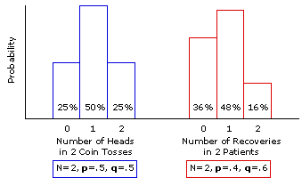
In Figure 6.1 we display these two sets of probabilities side-by-side in the form of two histograms. In each case, you can think of the total area of the histogram as representing 100% of the total probability that applies to that particular situation. Thus, for both examples there is a 100% chance that the outcome will include either zero or 1 or 2 of the particular events in question—heads or patient recoveries. All that differs is the way in which the 100% total is divided up by the 3 possible outcomes:25%|50%|25% for the coin-toss example versus 36%|48%|16% for the patient-recovery example.
Figure 6.1. Two Binomial Sampling Distributions for the Case where N=2
These two sets of probabilities are illustrative of a large class of theoretical structures collectively known as probability sampling distributions, so named because they describe the probabilities for the entire range of outcomes that are possible in the particular situations that are under consideration.
Thus, the sampling distribution for the coin-toss situation (N=2, p=.5, q=.5) specifies that any particular randomly selected sample of 2 tossed coins has a 25% chance of including zero heads, a 50% chance of including exactly 1 head, and a 25% chance of including 2 heads. The sampling distribution for the patient-recovery situation (N=2, p=.4, q=.6) specifies that any particular sample of 2 randomly selected patients who have come down with this disease has a 36% chance of ending up with zero recoveries, a 48% chance of ending up with exactly 1 recovery, and a 16% chance of ending up with 2 recoveries. By extension, these two sampling distributions would also specify that any particular randomly selected sample of 2 tossed coins has a 50%+25%=75% chance of including at least 1 head, and that any particular sample of 2 randomly selected patients has a 48%+16%=64% chance of ending up with at least one recovery.
Another way of interpreting a probability sampling distribution would be to say that it describes the manner in which the outcomes of any large number of randomly selected samples will tend to be distributed. Thus, a large number of randomly selected samples of 2 tossed coins would tend to have 25% of the samples including zero heads, 50% including exactly 1 head, and 25% including 2 heads. A large number of randomly selected 2-patient samples would tend to have 36% of the samples with zero recoveries, 48% with exactly 1 recovery, and 16% with 2 recoveries.
The interpretation of central tendency and variability for a sampling distribution is essentially the same as for any other distribution. The central tendency of the distribution describes the average of all the outcomes, and its variability is the measure of the tendency of individual outcomes to be dispersed away from that average. For the particular case of a binomial probability sampling distribution, these parameters can be easily determined according to the formulas given below. [Note the new symbols used here. When referring to an entire population of potential outcomes, the convention is to use (lower-case Greek letter "mu") for the mean and
  (lower-case Greek letter "sigma") for the variance and standard deviation.]
mean:  = Np
= Np
variance: 2 = Npq
standard deviation: = sqrt[Npq]
Thus, for the coin-toss example, with N=2, p=.5, and q=.5, you have
mean:  = 2x.5 = 1.0
variance: 2 = 2x.5x.5 = 0.5
standard deviation: = sqrt[0.5] = ±0.71
And for the patient-recovery example, with N=2, p=.4, and q=.6, you have
mean:  = 2x.4 = 0.8
variance: 2 = 2x.4x.6 = 0.48
standard deviation: = sqrt[0.48] = ±0.69
Although we are illustrating these various points about probability sampling distributions with the specific examples of coin tosses and patient recoveries, please keep in mind as we proceed that these distributions are abstract and general, in the sense that they apply to any probability situation at all that has certain defining properties. Thus, the sampling distribution shown in the left-hand histogram of Figure 6.1 is not limited to the example of tossing two coins. It applies to any situation at all in which the probability of a certain event isp=.5, the complementary probability of its non-occurrence is q=.5, and there are N=2 opportunities for it to occur. Similarly, the sampling distribution shown in the right-hand histogram of Figure 6.1 applies to any situation at all in which the defining properties are p=.4, q=.6, and N=2.
At any rate, in examining Figure 6.1 you can hardly fail to notice that the two sampling distributions have rather different shapes. Both are unimodal, but whereas the one for the coin-toss situation(p=.5, q=.5) is symmetrical, the one for the patient-recovery example (p=.4, q=.6) has a pronounced positive skew. But now see what happens when the size of the sample is increased from N=2 to N=10. The specific probabilities for the outcomes depicted by the histogram columns in Figure 6.2 have been calculated using the factorial and exponential formula examined in Chapter 5,
substituting N=10 along with the appropriate values of p, q, and k.
Figure 6.2. Two Binomial Sampling Distributions for the Case where N=10
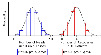
Please take a moment to compare the outlines of Figure 6.2 with those of Figure 6.1, for the transformation is quite remarkable. As a result of increasing the size of the sample to N=10, both sampling distributions have grown smoother, and the one for the patient-recovery example has in addition grown much more symmetrical. You will also surely recognize the smooth curve that has been superimposed upon the two sampling distributions in Figure 6.2 as the by-now familiar outline of the normal distribution.
In Figure 6.3 we increase the size of the sample to N=20, and there you can see these trends carried even further. The principle illustrated by Figures 6.1, 6.2, and 6.3 is that, as the size of N increases, the shape of a binomial sampling distribution comes closer and closer to the shape of the normal distribution. Eventually it comes so close as to be equivalent to the normal distribution, for all practical purposes—and that is the point where all the jagged complexity that we have been describing suddenly gives way to a smooth, streamlined simplicity. The reason for this remarkable convergence is explained in SideTrip 6.1
Figure 6.3. Two Binomial Sampling Distributions for the Case where N=20
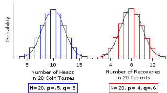
If the elemental probabilities, p and q, are both equal to .5, as in the coin-toss example, a sufficiently close approximation to the normal distribution is reached at the point where N is equal to 10. If p and q are anything other than .5, it is reached at some point beyond N=10. In general, a binomial sampling distribution may be regarded as a sufficiently close approximation to the normal distribution if the products of Np and Nq are both equal to or greater than 5. That is
For elemental probabilities of .4 and .6, as in our patient-recovery example, the point of sufficiently close approximation is reached at N=13; for .3 and .7, it is reached at N=17; for .2 and .8, it is reached at N=25; and so on. The simple way of determining these points is to divide 5 by either p or q, whichever is smaller, rounding the result up to the next higher integer if it comes out with a decimal fraction. Thus, for .4 and .6 you have5/.4=12.5, which rounds up to N=13; for .3 and .7 it is 5/.3=16.67, which rounds up to N=17; and so on.
The graph of the normal distribution that appears in Figure 6.4 will help you see where all this is leading. Once you know that a distribution is normal, or at least a close approximation of the normal, you are then in a position to specify the proportion of the distribution that falls to the left or right of any particular point along the horizontal axis, or alternatively the proportion that falls in-between any two points along the horizontal axis. And specifying the proportion is tantamount to specifying the probability. For the standardized normal distribution, these points along the horizontal axis are marked out in units of z, with each unit of z being equal to 1 unit of standarddeviation,  .
.
Figure 6.4. The Unit Normal Distribution
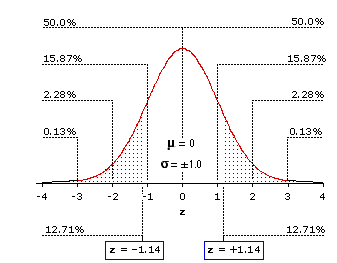
Most of the percentage values that appear in the body of the graph will already be familiar to you. To the right ofz=+1 falls 15.87% of the total distribution; to the right of z=+2 falls 2.28% of the total distribution; and so on. And since the normal distribution is precisely symmetrical, the same percentages also fall to the left of corresponding negative values of z. For reasons that will be evident in a moment, Figure 6.4 also shows shaded areas corresponding to the proportions of the normal distribution that fall to the left of z=—1.14 and to the right of z=+1.14— in each case, 12.71%. An abbreviated version of the standard table of the normal distribution is shown in Table 6.1. The complete version is given in Appendix A. (Please note that the entries in Table 6.1 are not listed as percentages but as proportions; e.g., .1587 instead of 15.87%.)
Table 6.1. Proportions of the normal distribution falling to the left of negative values of z or to the right of positive values of z. Bold-face entries pertain to examples discussed in the text.
Now turn to Figure 6.5 where you will see this same standardized normal distribution superimposed on the binomial sampling distribution that applies to our patient-recovery example with a sample size of 20. The defining properties of this sampling distribution are N=20,p=.4, q=.6. Hence
mean:  = 20x.4 = 8.0
standard deviation: = sqrt[20x.4x.6] = ±2.19
Figure 6.5. Binomial Sampling Distribution for N=20, p=.4, q=.6
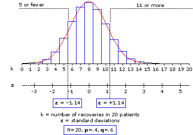
You will note that there are two scales along the horizontal axis of Figure 6.5. The first, labeled k, delineates "number of recoveries in 20 patients"; and the second, labeled z, is a direct translation of this binomial k scale into units of standard deviation, with each unit of standard deviation equal to±2.19 units of k. Any particular one of the discrete values on the k scale—0, 1, 2, ... , 18, 19, 20—can be directly translated into its corresponding value on the z scale by application of the formula
Thus, for k=5 we have
and for k=11:
With the calculation of z for a binomial outcome of the general type "k or fewer" or "k or more," you are then in a position to use the normal distribution for assessing the probability associated with that outcome. You simply treat your calculated value of z as though it belonged to the z scale of the normal distribution—and read off the corresponding probability value from the table of the normal distribution. The two particular values of z that we have just calculated arez=—1.14 for "5 or fewer" recoveries and z=+1.14 for "11 or more" recoveries. As we saw a moment ago in Figure 6.5 and Table 6.1, the proportions of the normal distribution falling to the left of z=—1.14 and to the right of z=+1.14 are in each case equal to .1271. Hence, on the basis of the normal distribution we would judge that with a random sample of 20 patients there is a 12.71% chance that as few as 5 will spontaneously recover, and an equal 12.71% chance that as many as 11 will spontaneously recover. If you work out the exact binomial probabilities for these two outcomes using the factorial and exponential formula given earlier, you will find that they come out to 12.56% for "5 or fewer" and 12.75% for "11 or more." The 12.71% probability values arrived at via the normal distribution do not hit these targets precisely, but for all practical purposes they are close enough. The difference between .1271 and .1256 is only .0015; between .1271 and .1275 it is only .0004.
To appreciate just how useful and labor-saving this streamlining can be, return for a moment to the second experiment of our medical researchers, the one in which there were 430 recoveries out of 1,000 patients. The question is: In a random sample of 1,000 patients, how likely is it that as many as 430(k>430) would recover by mere chance, if the plant extract had no effectiveness whatsoever? First try to imagine how much it would cost you in time and patience to perform the requisite 571 exact binomial calculations according to the factorial and exponential formula, assuming you had access to a calculator powerful enough to perform huge operations such as 1,000! and .4430x.6570— and then reflect on how very much easier it is to reach the same goal on the basis of the normal distribution.
First establish the defining properties of the relevant binomial sampling distribution, making sure that the products of Np and Nq are both equal to or greater than 5:
N=1,000, p=.4, q=.6. Hence
mean: = 1,000x.4 = 400
standard deviation: = sqrt[1,000x.4x.6] = ±15.49
Then perform the simple calculation that translates the details of the binomial situation into the language of the normal distribution:
And then refer your calculated value of z to the table of the normal distribution. For the moment you need only refer to the abbreviated version shown in Table 6.1, where you will find that the proportion of the normal distribution falling to the right ofz=+1.9 is equal to .0287.
The meaning of this proportion is illustrated in Figure 6.6. Of all the possible spontaneous-recovery outcomes that could have occurred within this sample—zero recoveries, 1 recovery, 2 recoveries, and so on—only 2.87% would include as many as 430 recoveries. The mere-chance probability of the observed result is thereforeP=.0287, which of course clears the conventional cut-off point for statistical significance (P<.05) by a considerable margin.
Figure 6.6. Location of z=+1.90 within the Unit Normal Distribution
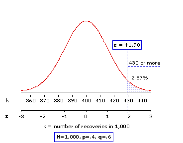
Moving beyond the rather rigid mechanics of the .05 criterion of statistical significance, you can also think of thisP=.0287 probability value in terms of confidence. There is only about a 3% likelihood that the observed outcome would have occurred by mere chance coincidence. Hence, you can be about 97% confident that it is the result of something other than mere chance coincidence—presumably some active ingredient of the plant extract. The researchers can now go on to the costly task of isolating and refining that ingredient, with a high degree of confidence that they are on the right track.
As we indicated earlier, the streamlining of binomial probabilities was only the first historical step. In the course of time there came the discovery and detailed analysis of several other families of sampling distributions, each providing a relatively simple streamlined method for answering inferential-statistical questions of the general type: How likely is it that such-and-such might occur by mere chance coincidence? In the remaining chapters of this text we will be making extensive use of some of these families of sampling distributions, in particular, several that are variations on the normal distribution, plus some others that are known ast-distributions, F-distributions, and chi-square distributions. Of all of these, it is the family of chi-square sampling distributions whose logic follows most closely upon the concepts we have been developing in the present chapter, so that is where we will go next, in Chapter 8. First, however, in Chapter 7, another brief interlude on the general concept of statistical significance.
| p | the probability that the event or outcome in question will occur in any particular instance | E.g., | q | the probability that the event or outcome in question will not occur in any particular instance | E.g., | N | the number of instances in which the event or outcome has the opportunity to occur |
| |
To show how the streamlining came about, we will begin by considering the very simple binomial probability situation in which N is equal to 2, and then work our way up through some more complex binomial situations. If you are tossing 2 coins with elemental probabilities of
| Coin | Sub-pathway Probability | Number of Heads | Main Pathway Probability A | B | -- | -- | .5x.5=.25 | 0 | .25 | (25%) | -- | H H | -- .5x.5=.25 | .5x.5=.25 1 | .50 | (50%) | H | H | .5x.5=.25 | 2 | .25 | (25%) | Totals | 1.0 | (100%) | | |||||
Similarly, if you are considering 2 randomly selected patients with elemental probabilities of
| Patient | Sub-pathway Probability | Number of Recoveries | Main Pathway Probability A | B | -- | -- | .6x.6=.36 | 0 | .36 | (36%) | -- | R R | -- .6x.4=.24 | .4x.6=.24 1 | .48 | (48%) | R | R | .4x.4=.16 | 2 | .16 | (16%) | Totals | 1.0 | (100%) | | |||||
In Figure 6.1 we display these two sets of probabilities side-by-side in the form of two histograms. In each case, you can think of the total area of the histogram as representing 100% of the total probability that applies to that particular situation. Thus, for both examples there is a 100% chance that the outcome will include either zero or 1 or 2 of the particular events in question—heads or patient recoveries. All that differs is the way in which the 100% total is divided up by the 3 possible outcomes:
Figure 6.1. Two Binomial Sampling Distributions for the Case where N=2

These two sets of probabilities are illustrative of a large class of theoretical structures collectively known as probability sampling distributions, so named because they describe the probabilities for the entire range of outcomes that are possible in the particular situations that are under consideration.
Following this chapter is an appendix that will dynamically generate the graphical outlines and numerical details of the binomial sampling distribution for any values of p and q, and for any value of N between 1 and 40, inclusive. |
Another way of interpreting a probability sampling distribution would be to say that it describes the manner in which the outcomes of any large number of randomly selected samples will tend to be distributed. Thus, a large number of randomly selected samples of 2 tossed coins would tend to have 25% of the samples including zero heads, 50% including exactly 1 head, and 25% including 2 heads. A large number of randomly selected 2-patient samples would tend to have 36% of the samples with zero recoveries, 48% with exactly 1 recovery, and 16% with 2 recoveries.
The interpretation of central tendency and variability for a sampling distribution is essentially the same as for any other distribution. The central tendency of the distribution describes the average of all the outcomes, and its variability is the measure of the tendency of individual outcomes to be dispersed away from that average. For the particular case of a binomial probability sampling distribution, these parameters can be easily determined according to the formulas given below. [Note the new symbols used here. When referring to an entire population of potential outcomes, the convention is to use
variance:
standard deviation:
Thus, for the coin-toss example, with N=2, p=.5, and q=.5, you have
variance:
standard deviation:
And for the patient-recovery example, with N=2, p=.4, and q=.6, you have
variance:
standard deviation:
Although we are illustrating these various points about probability sampling distributions with the specific examples of coin tosses and patient recoveries, please keep in mind as we proceed that these distributions are abstract and general, in the sense that they apply to any probability situation at all that has certain defining properties. Thus, the sampling distribution shown in the left-hand histogram of Figure 6.1 is not limited to the example of tossing two coins. It applies to any situation at all in which the probability of a certain event is
At any rate, in examining Figure 6.1 you can hardly fail to notice that the two sampling distributions have rather different shapes. Both are unimodal, but whereas the one for the coin-toss situation
|
P(k out of N) = |
N! k!(N—k)! | x |
pk x qN-kT |
Figure 6.2. Two Binomial Sampling Distributions for the Case where N=10

Please take a moment to compare the outlines of Figure 6.2 with those of Figure 6.1, for the transformation is quite remarkable. As a result of increasing the size of the sample to N=10, both sampling distributions have grown smoother, and the one for the patient-recovery example has in addition grown much more symmetrical. You will also surely recognize the smooth curve that has been superimposed upon the two sampling distributions in Figure 6.2 as the by-now familiar outline of the normal distribution.
In Figure 6.3 we increase the size of the sample to N=20, and there you can see these trends carried even further. The principle illustrated by Figures 6.1, 6.2, and 6.3 is that, as the size of N increases, the shape of a binomial sampling distribution comes closer and closer to the shape of the normal distribution. Eventually it comes so close as to be equivalent to the normal distribution, for all practical purposes—and that is the point where all the jagged complexity that we have been describing suddenly gives way to a smooth, streamlined simplicity. The reason for this remarkable convergence is explained in SideTrip 6.1
Figure 6.3. Two Binomial Sampling Distributions for the Case where N=20

If the elemental probabilities, p and q, are both equal to .5, as in the coin-toss example, a sufficiently close approximation to the normal distribution is reached at the point where N is equal to 10. If p and q are anything other than .5, it is reached at some point beyond N=10. In general, a binomial sampling distribution may be regarded as a sufficiently close approximation to the normal distribution if the products of Np and Nq are both equal to or greater than 5. That is
| Np>5 and Nq>5 |
Criterion for determining that a binomial sampling distribution is a sufficiently close approximation of the normal distribution. |
For elemental probabilities of .4 and .6, as in our patient-recovery example, the point of sufficiently close approximation is reached at N=13; for .3 and .7, it is reached at N=17; for .2 and .8, it is reached at N=25; and so on. The simple way of determining these points is to divide 5 by either p or q, whichever is smaller, rounding the result up to the next higher integer if it comes out with a decimal fraction. Thus, for .4 and .6 you have
The graph of the normal distribution that appears in Figure 6.4 will help you see where all this is leading. Once you know that a distribution is normal, or at least a close approximation of the normal, you are then in a position to specify the proportion of the distribution that falls to the left or right of any particular point along the horizontal axis, or alternatively the proportion that falls in-between any two points along the horizontal axis. And specifying the proportion is tantamount to specifying the probability. For the standardized normal distribution, these points along the horizontal axis are marked out in units of z, with each unit of z being equal to 1 unit of standard
Figure 6.4. The Unit Normal Distribution

Most of the percentage values that appear in the body of the graph will already be familiar to you. To the right of
Table 6.1. Proportions of the normal distribution falling to the left of negative values of z or to the right of positive values of z. Bold-face entries pertain to examples discussed in the text.
| ±z 0.00 0.20 0.40 0.60 0.80 1.00 1.14 1.20 1.40 1.60 | Area Beyond ±z .5000 .4702 .3446 .2743 .2119 .1587 .1271 .1151 .0808 .0548 | ±z 1.80 1.90 2.00 2.20 2.40 2.60 2.80 3.00 3.50 4.00 | Area Beyond ±z .0359 .0287 .0228 .0139 .0082 .0047 .0026 .0013 .0002 .00003
| | |||||||
Now turn to Figure 6.5 where you will see this same standardized normal distribution superimposed on the binomial sampling distribution that applies to our patient-recovery example with a sample size of 20. The defining properties of this sampling distribution are N=20,
standard deviation:
Figure 6.5. Binomial Sampling Distribution for N=20, p=.4, q=.6

You will note that there are two scales along the horizontal axis of Figure 6.5. The first, labeled k, delineates "number of recoveries in 20 patients"; and the second, labeled z, is a direct translation of this binomial k scale into units of standard deviation, with each unit of standard deviation equal to
| z = | (k— | Note 1. Only the positive value of Note 2. The component ±.5 ('plus or minus .5') in the numerator is a 'correction for continuity', aimed at transforming the zig-zag angularity of the binomial distribution into the smooth curve of the normal distribution. It achieves this effect by reducing the distance between k and the mean by one-half unit. Thus, when k is smaller than the mean you add half a
| | |||
Thus, for k=5 we have
| z = | (5—8 )+.5 2.19 | = | —2.5 2.19 | = —1.14 |
and for k=11:
| z = | (11—8 )—.5 2.19 | = | +2.5 2.19 | = +1.14 |
With the calculation of z for a binomial outcome of the general type "k or fewer" or "k or more," you are then in a position to use the normal distribution for assessing the probability associated with that outcome. You simply treat your calculated value of z as though it belonged to the z scale of the normal distribution—and read off the corresponding probability value from the table of the normal distribution. The two particular values of z that we have just calculated are
To appreciate just how useful and labor-saving this streamlining can be, return for a moment to the second experiment of our medical researchers, the one in which there were 430 recoveries out of 1,000 patients. The question is: In a random sample of 1,000 patients, how likely is it that as many as 430
First establish the defining properties of the relevant binomial sampling distribution, making sure that the products of Np and Nq are both equal to or greater than 5:
mean:
standard deviation:
Then perform the simple calculation that translates the details of the binomial situation into the language of the normal distribution:
| z = | (430—400 )—.5 15.49 | = | +29.5 15.49 | = +1.90 |
And then refer your calculated value of z to the table of the normal distribution. For the moment you need only refer to the abbreviated version shown in Table 6.1, where you will find that the proportion of the normal distribution falling to the right of
The meaning of this proportion is illustrated in Figure 6.6. Of all the possible spontaneous-recovery outcomes that could have occurred within this sample—zero recoveries, 1 recovery, 2 recoveries, and so on—only 2.87% would include as many as 430 recoveries. The mere-chance probability of the observed result is therefore
Figure 6.6. Location of z=+1.90 within the Unit Normal Distribution

Moving beyond the rather rigid mechanics of the .05 criterion of statistical significance, you can also think of this
As we indicated earlier, the streamlining of binomial probabilities was only the first historical step. In the course of time there came the discovery and detailed analysis of several other families of sampling distributions, each providing a relatively simple streamlined method for answering inferential-statistical questions of the general type: How likely is it that such-and-such might occur by mere chance coincidence? In the remaining chapters of this text we will be making extensive use of some of these families of sampling distributions, in particular, several that are variations on the normal distribution, plus some others that are known as
This chapter includes two appendices:
|
End of Chapter 6.
Return to Top of Chapter 6
Go to Chapter 7 [Tests of Statistical Significance: Three Overarching Concepts]
| Home | Click this link only if the present page does not appear in a frameset headed by the logo Concepts and Applications of Inferential Statistics |