[If you have already read this introduction or wish to skip it, click here and enter the number of time periods at the prompt.]
Suppose that 100 subjects of a certain type were tracked over a period of time to determine how many survived for one year, two years, three years, and so forth. If all the subjects remained accessible throughout the entire length of the study, the estimation of year-by-year survival probabilities for subjects of this type in general would be an easy matter. The survival of 87 subjects at the end of the first year would give a one-year survival probability estimate of
But in real-life longitudinal research it rarely works out this neatly. Typically there are subjects lost along the way for reasons unrelated to the focus of the study. To illustrate the complication in this sort of situation, consider the following hypothetical scenario. Of the 100 subjects who are "at risk" at the beginning of the study, 3 become unavailable during the first year and 5 are known to have died by the end of the first year. Another 3 become unavailable during the second year and another 10 are known to have died by the end of the second year. And so on for the other years shown. For the sake of numerical simplicity I am showing 3 subjects becoming unavailable in each of the five years. In real-life research the loss rate would of course not normally be so uniform as this.
| Time Period | At Risk | Became Unavailable (Censored) | Died | Survived| Year 1 | 100 | 3 | 5 | ? | Year 2 | ? | 3 | 10 | ? | Year 3 | ? | 3 | 15 | ? | Year 4 | ? | 3 | 20 | ? | Year 5 | ? | 3 | 25 | ? | |
Kaplan and Meier, recognizing that any attempt to salvage this information would involve a certain amount of "fudging," proposed that subjects who become unavailable during a given time period be counted among those who survive through the end of that period, but then deleted from the number who are at risk for the next time period. "These conventions," they wrote,
| may be paraphrased by saying that deaths recorded as of |
| Time Period | At Risk | Became Unavailable (Censored) | Died | Survived| Year 1 | 100 | 3 | 5 | 95 | Year 2 | 92 | 3 | 10 | 82 | Year 3 | 79 | 3 | 15 | 64 | Year 4 | 61 | 3 | 20 | 41 | Year 5 | 38 | 3 | 25 | 13 | |
As illustrated in the next table, the Kaplan-Meier procedure then calculates the survival probability estimate for each of the t time periods, except the first, as a compound conditional probability.
| Time Period | At Risk | Became Unavailable (Censored) | Died | Survived | Kaplan-Meier Survival Probability Estimate| Year 1 | 100 | 3 | 5 | 95 | (95/100)=0.95 | Year 2 | 92 | 3 | 10 | 82 | (95/100)x(82/92)=0.8467 | Year 3 | 79 | 3 | 15 | 64 | (95/100)x(82/92)x(64/79)=0.70 | Year 4 | 61 | 3 | 20 | 41 | (95/100)x(82/92)x(64/79)x(41/61)=0.4611 | Year 5 | 38 | 3 | 25 | 13 | (95/100)x(82/92)x(64/79)x(41/61)x(13/38)=0.1577 | |
The estimate for surviving through
This cumbersome structure is shown only to illustrate the logic of the procedure. For practical computational purposes, the same results can be obtained more efficiently by using the Kaplan-Meier product-limit estimatorQ
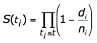
where S(ti) is the estimated survival probability for any particular one of the t time periods;
The Kaplan-Meier procedure is not limited to the measurement of survival in the narrow sense of dying or not dying. It can also be used to estimate the time-defined probabilities for the failure of an instrument or device of a certain type; or alternatively, to estimate the time-defined probabilities for some particular type of success (e.g., finding employment after becoming unemployed).
For purposes of illustration, the following Kaplan-Meier calculator is set up for 5 time periods and the values that need to be entered for the above example (total number of subjects along with the number of subjects for each time period who died or became unavailable) are already in place. To perform the analysis on the data of this example, click the «Calculate» button. To perform an analysis on a different set of data with exactly 5 time periods, click the «Clear» button, enter the relevant values into the yellow cells, and then click «Calculate». To perform an analysis with fewer or more than 5 time periods, click the «Reload» button and enter the number of time periods at the prompt. The user's own labels for the time periods can be substituted for the labels t1, t2, etc.
c
Data EntryQ|
| Time | Period At Risk | Became | Unavailable (Censored) Died | (Failed) (Succeeded) Survival | Probability Estimate 0.95 Confidence Interval | Lower Limit | Upper Limit | | ||||||||||||||
method (corrected for continuity) described by Robert
by
References:Kaplan, E.L. & Meier, P. "Nonparametric estimation from incomplete observations," Journal of the American Statistical Association, 53, 457-481 (1958).
Newcombe, Robert G. "Two-Sided Confidence Intervals for the Single Proportion: Comparison of Seven Methods," Statistics in Medicine, 17, 857-872 (1998).
Wilson, E. B. "Probable Inference, the Law of Succession, and Statistical Inference," Journal of the American Statistical Association, 22, 209-212 (1927).
| Home | Click this link only if you did not arrive here via the VassarStats main page. |
©Richard Lowry 2001-
All rights reserved.