Simple ROC Curve Analysis
|
If you have visited this page before and wish to skip the preamble, click here to go directly to the calculator. |
The programming on this page provides a streamlined approach to ROC curve analysis that I think will be fairly accessible to the non-statistician. For the more heavy-duty version of this procedure, applicable software can be downloaded from the Department of Radiology, Kurt Rossmann Laboratories, University of Chicago.
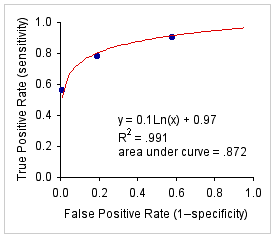
To illustrate, consider the following set of data (source). Of a total of 125 subjects, 32 are known to be hypothyroid and 93 are known to have normal thyroid function. All subjects are assessed with respect to T4 (thyroxine) levels, and then sorted among the four ordinal categories: T4<5.1, T4=5.1 to 7.0, T4=7.1 to 9.0, and T4>9.0. Of the 19 subjects with T4 levels lower than 5.1, 18 were in fact hypothyroid while only 1 was euthyroid. Thus, if a T4 of 5 or less were taken as an indication of hypothroidism, this measure would yield 18 true positives and 1 false positive, with a true-positive rate (sensitivity) of 18/32=.5625 and a false-positive rate (1-specificity) of 1/93=.0108.
| Observed Frequencies | Cumulative Rates| T4 Value | Diagnostic Level Euthyroid | False Positive Hypothyroid | True Positive Euthyroid | False Positive Hypothyroid | True Positive <5.1 | 1 | 18 | .0108 | .5625 | 5.1-7.0 | 17 | 7 | .1935 | .7813 | 7.1-9.0 | 36 | 4 | .5806 | .9063 | >9.0 | 39 | 3 | 1.0 | 1.0 | Totals: | 93 | 32 | | |||
Similarly, 7 of the hypothyroid subjects and 17 of the euthyroid had T4 levels between 5.1 and 7.0. Thus, if any value of T4 less than 7.1 were taken as an indication of hypothroidism, this measure would yield 18+7=25 true positives and 1+17=18 false positive, with a true-positive rate of 25/32=.7813 and a false-positive rate of 18/93=.1935. And so on for the other diagnostic levels, T4=7.1 to 9.0, and T4>9.0.
Given k exhaustive ordinal diagnostic levels, the programming on this page fits a simple logarithmic curve to the first k-1 pairs of cumulative rates, with
x = cumulative false-positive rate| y = cumulative true-positive rate | |
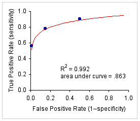
| A. Example data fitted by a simple A. logarithmic curve. | B. Example data fitted by a binormal B. ROC curve.   |
To proceed, enter into the cells of the following table either the observed frequencies or the cumulative rates for each of the k diagnostic levels, up to a maximum of k=10. (Note that this procedure makes no sense with k<4.) If you are entering observed frequencies, cumulative rates will be calculated automatically. If you are entering cumulative rates, the final entry in each of the two columns on the right must always be equal to 1.0. Cumulative rates can be entered as either decimal fractions (.5625) or common fractions (18/32). When all values have been entered, click the «Calculate» button, and the results of the analysis will appear in the scrolling text box that follows the data- entry table.
To illustrate further the details of data entry, click one or another of the following lines to enter the data of the above example
as observed frequencies| as cumulative rates (decimal fractions) | as cumulative rates (common fractions) | |
| Diagnostic Level | Observed Frequencies | Cumulative Rates False | Positive True | Positive False | Positive True | Positive | |||
|
Click this button to place a printable version of the fitted curve in a separate window. | |
|
| | ||||||
| Home | Click this link only if you did not arrive here via the VassarStats main page. |
©Richard Lowry 2001-
All rights reserved.