Simple Logistic Regression

If you have visited this page before and wish to skip the preamble, click here to go directly to the calculator.

The following table shows the relationship, for 64 infants, between

	X:	gestational age of the infant (in weeks) at the time of birth [column (i)]; and
	Y:	whether the infant was breast feeding at the time of release from hospital ["no" coded as "0" and entered in column (ii); "yes" coded as "1" and entered in column (iii)]

Also shown in the table are

	(v)	the observed probability of Y=1 for each level of X, calculated as the ratio of the number of instances of Y=1 to the total number of instances of Y for that level;
	(vi)	the odds for each level of X, calculated as the ratio of the number of Y=1 entries to the number of Y=0 entries for each level, or alternatively as

observed probability

(1 - observed probability)

	and
	(vii)	the natural logarithm of the odds for each level of X, designated as "log odds."

i	ii	iii	iv	v	vi	vii
X	Instances of Y Coded as		Total ii+iii	Y as Observed Probability	Y as Odds	Y as Log Odds
X	0	1	Total ii+iii	Y as Observed Probability	Y as Odds	Y as Log Odds
28 29 30 31 32 33	4 3 2 2 4 1	2 2 7 7 16 14	6 5 9 9 20 15	.3333 .4000 .7778 .7778 .8000 .9333	.5000 .6667 3.5000 3.5000 4.0000 14.0000	-.6931 -.4055 1.2528 1.2528 1.3863 2.6391

Graph A, below, shows the linear regression of the observed probabilities, Y, on the independent variable X. The problem with ordinary linear regression in a situation of this sort is evident at a glance: extend the regression line a few units upward or downward along the X axis and you will end up with predicted probabilities that fall outside the legitimate and meaningful range of 0.0 to 1.0, inclusive. Logistic regression, as shown in Graph B, fits the relationship between X and Y with a special S-shaped curve that is mathematically constrained to remain within the range of 0.0 to 1.0 on the Y axis.

A. Ordinary Linear Regression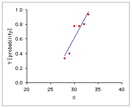

B. Logistic Regression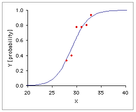

The mechanics of the process begin with the log odds, which will be equal to 0.0 when the probability in question is equal to .50, smaller than 0.0 when the probability is less than .50, and greater than 0.0 when the probability is greater than .50. The form of logistic regression supported by the present page involves a simple weighted linear regression of the observed log odds on the independent variable X. As shown below in Graph C, this regression for the example at hand finds an intercept of -17.2086 and a slope of .5934.

X	Observed Probability	Log Odds	Weight	C. Weighted Linear Regression of C. Observed Log Odds on X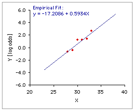
28 29 30 31 32 33	.3333 .4000 .7778 .7778 .8000 .9333	-.6931 -.4055 1.2528 1.2528 1.3863 2.6391	6 5 9 9 20 15
For each level of X, the weighting factor is the number of observations for that level.
Intercept=-17.2086 is the point on the Y-axis (log odds) crossed by the regression line when X=0. Slope=.5934 is the rate at which the predicted log odds increases (or, in some cases, decreases) with each successive unit of X. Within the context of logistic regression, you will usually find the slope of the log odds regression line referred to as the "constant." The exponent of the slope exp(.5934) = 1.81 describes the proportionate rate at which the predicted odds changes with each successive unit of X. In the present example, the predicted odds for X=29 is 1.81 times as large as the one for X=28; the one for X=30 is 1.81 times as large as the one for X=29; and so on.

Once this initial linear regression is obtained, the predicted log odds for any particular value of X can then be translated back into a predicted probability value. Thus, for X=31 in the present example, the predicted log odds would be

log[odds] = -17.2086+(.5934x31) = 1.1868

The corresponding predicted odds would be

odds = exp(log[odds]) = exp(1.1868)=3.2766

And the corresponding predicted probability would be

probability = odds/(1+odds)=3.2766/(1+3.2766) = .7662

Perform this translation throughout the range of X values and you go from the straight line of the graph on the left to the S-shaped curve of the logistic regression on the right.

Please note, however, that the logistic regression accomplished by this page is based on a simple, plain-vanilla empirical regression. You will typically find logistic regression procedures framed in terms of an abstraction known as the maximized log likelihood function. For two reasons, this page does not follow that procedure. The first reason, which can be counted as either a high-minded philosophical reservation or a low-minded personal quirk, is that the maximized log likelihood method has always impressed me as an exercise in excessive fine-tuning, reminiscent on some occasions of what Alfred North Whitehead identified as the fallacy of misplaced concreteness,

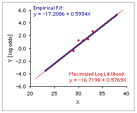and on others of what Freud described as the narcissism of small differences. The second reason is that in most real-world cases there is little if any practical difference between the results of the two methods. The blue line in the adjacent graph is the same empirical regression line described above; the red line shows the regression resulting from the method of maximized log likelihood. I find it difficult to suppose that the fine-tuned abstraction of the latter is saying anything very different from what is being said by the former.

At any rate, Calculator 1, below, will perform a plain-vanilla empirical logistic regression of the sort just described, while Calculator 2, based on that regression, will fetch the predicted probability and odds associated with any particular value of X.

Data Entry:

X	Instances of Y Coded as		Enter the values of X into the designated cells. beginning with the top-most cell. Then, for each level of X, enter the number of instances coded as 0 and 1. When all values have been entered, click the «Calculate 1» button. Note that all entries in the "0" and "1" cells associated with an entered value of X must be positive integers greater than zero. If a zero is entered into any of these cells, it will be replaced by "1" and the adjacent cell will be incremented by 1. For an illustration of data entry, click here to enter the data described in the introductory example.
	0	1

For weighted linear regression of log odds on X:

intercept:
slope:
exp(slope):
R²:

X	Probabilities		Odds
X	Observed	Predicted	Observed	Predicted

X	Predicted		To calculate the predicted probability and odds for any particular value of X, enter X into the designated cell, then click the «Calculate 2» Button.
	Probability	Odds

Home

Click this link only if you did not arrive here via the VassarStats main page.