Correlation for Unordered Pairs
Eta2, Three Intercorrelated Variables: Intraclass Correlation,
 & Resampling of r
Click here if you have visited this page before and wish to skip the introduction.
The assessment of correlation via the familiar Pearson product-moment procedure applies only to those situations where one particular member of a bivariate pair of measures unequivocally belongs to the X variable and the other unequivocally belongs to the Y variable. The phrase "unordered pairs" refers to those cases in which the designation of either member of a pair as "X"or "Y," "A" or "B," "First" or "Second," etc., is entirely arbitrary.
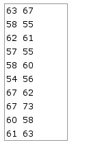
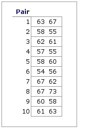 An example of unordered pairs is shown in the adjacent table, which lists the measures on a certain psychological variable for each of the members in each of 10 pairs of identical twins. The scores for Pair 1 are listed as
 63 67; it could just as easily have been 67 63. The same is true for each of the other pairs: it is entirely arbitrary which of the items within the pair is listed first and which is listed second. Nonetheless, examine these 10 pairings with the naked eye and you will clearly see the suggestion of a correlation. The higher the score of one of the twins of a pair, the higher tends to be the score of the other. Conversely, the lower the score of one, the lower tends to be the score of the other.
In situations of this sort, correlation can be measured by way of an analysis of variance procedure that is structurally identical with what is described elswhere on this site as one-way ANOVA for independent samples. The following table shows the same paired measures as above, except that now they are arrayed in a manner more readily recognizable as an analysis of variance format. Also shown here are the means for each of the 10 pairs.
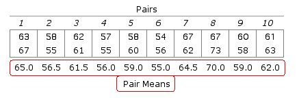
The logic of the procedure is this. If both members of a pair have relatively high values, the mean value for that pair will also be relatively high; and conversely, when both members of a pair have relatively low values, the mean for that pair will be relatively low. Hence, the greater the correlation, the greater will be the variability among the means of the pairs(a.k.a., between-groups variability) as a proportion of total variability, and the smaller will be the proportion of total variability that exists inside the pairs (a.k.a., within-groups variability).
The next table shows the results of an analysis of variance performed upon this data set, along with two measures of correlation for unordered pairs that can be derived from these results.
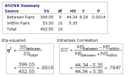
Both of these measures of correlation have the same level of statistical significance as theF-ratio of the ANOVA from which they derive. In the present example, that level is P=0.0014.
The interpretation ofeta2=.8818 is straightforward: of the total variability contained within the 20 measures in this data set, 88.18% reflects on-average differences among the 10 pairs of twins. Alternatively, you could say that 88.18% of the total variability reflects the tendency of the two twins within any particular pair to have approximately the same measures.
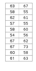
The precise meaning of the intraclass correlation coefficient is less readily stated in ordinary language. As an intuitive approximation, consider the following scenario. Each time you click the button below, labeled «Resample», one of the values within each of the 10 pairs is randomly designatedas X and the other as Y. In a set of 10 pairs of values, the total possible number of unique XY combinations would be 210=1,024. (With 20 pairs, 220=1,048,576; and so on.) Note also that these different combinations yield different values of r, the Pearson product-moment correlation coefficient.
The point of the illustration is this. For any particular set of N unordered pairs of values, there would be a total of 2N unique XY combinations. If you had the time and patience to compile these 2N combinations and then calculate the Pearson product-moment correlation coefficient for each and every one of them, you would find that the average of these 2N values of r would come out fairly close to what is much more easily calculated as the intraclass correlation coefficient.
However, do keep in mind that this is only an intuitive approximation of the meaning of the intraclass correlation coefficient. Actually, the present example is a good reminder of this caveat. The intraclass correlation coefficient here comes outas .7847, whereas the average of the 1,024 values of r is about .82. Fairly close, but certainly not exact. In addition to calculating eta2 and the intraclass correlation coefficient, the present page also has a "resampling" provision for gaining an idea of what would be the average r for the whole range of possible XY permutations.
Procedure
©Richard Lowry 2001-
All rights reserved.
Click here if you have visited this page before and wish to skip the introduction.
The assessment of correlation via the familiar Pearson product-moment procedure applies only to those situations where one particular member of a bivariate pair of measures unequivocally belongs to the X variable and the other unequivocally belongs to the Y variable. The phrase "unordered pairs" refers to those cases in which the designation of either member of a pair as "X"
An example of unordered pairs is shown in the adjacent table, which lists the measures on a certain psychological variable for each of the members in each of 10 pairs of identical twins. The scores for Pair 1 are listed as In situations of this sort, correlation can be measured by way of an analysis of variance procedure that is structurally identical with what is described elswhere on this site as one-way ANOVA for independent samples. The following table shows the same paired measures as above, except that now they are arrayed in a manner more readily recognizable as an analysis of variance format. Also shown here are the means for each of the 10 pairs.
The logic of the procedure is this. If both members of a pair have relatively high values, the mean value for that pair will also be relatively high; and conversely, when both members of a pair have relatively low values, the mean for that pair will be relatively low. Hence, the greater the correlation, the greater will be the variability among the means of the pairs
The next table shows the results of an analysis of variance performed upon this data set, along with two measures of correlation for unordered pairs that can be derived from these results.
Both of these measures of correlation have the same level of statistical significance as the
The interpretation of
The precise meaning of the intraclass correlation coefficient is less readily stated in ordinary language. As an intuitive approximation, consider the following scenario. Each time you click the button below, labeled «Resample», one of the values within each of the 10 pairs is randomly designated
|
| X | Y |
The point of the illustration is this. For any particular set of N unordered pairs of values, there would be a total of 2N unique XY combinations. If you had the time and patience to compile these 2N combinations and then calculate the Pearson product-moment correlation coefficient for each and every one of them, you would find that the average of these 2N values of r would come out fairly close to what is much more easily calculated as the intraclass correlation coefficient.
However, do keep in mind that this is only an intuitive approximation of the meaning of the intraclass correlation coefficient. Actually, the present example is a good reminder of this caveat. The intraclass correlation coefficient here comes out
Procedure
- Importing Data via Copy & Paste:T
 When importing data from a spreadsheet, the paired values must be in the form of two adjacent columns. Within the spreadsheet application, select and copy the two columns of data. Then return to this page, click the cursor into the data-entry field and perform the 'Paste' operation.T
- Direct Entry into Data Field:T
 Click the cursor into the empty data-entry field, enter the first value of Pair 1; then press the space bar one (and only one) time; then enter the second value of Pair 1; then press the carriage return key. Do the same for subsequent paired values, except that the final entry should not be followed by a carriage return.T
- Data Check:T
Make sure that the final line in the data-entry field is not followed by a carriage return. (An extra carriage return at the end of the list will be interpreted as an extra data entry whose value is zero. Importing data via the copy and paste procedure will almost always produce an extra carriage return at the end of a column.) After the bivariate list has been pasted into the data-entry field, click the cursor immediately to the right of the final entry in the list, then press the down-arrow key. If an extra line is present, the cursor will move downward. Extra lines can be removed by pressing the down arrow key until the cursor no longer moves, and then pressing the 'Backspace' key (on a Mac platform, 'delete') until the cursor stands immediately to the right of the final entry.T
- After verification of data entry, click the button labeled «Calculate». If you are using the resampling provision, be sure to click the «Calculate» button first. To get the best approximation of the true average value of r, continue resampling until the observed value of
"Average r" stabilizes. The greater the number of pairs, the longer each resampling will take. 1,000 resamplings will take 10 times as long as 100.
| Data Entry: |
| Home | Click this link only if you did not arrive here via the VassarStats main page. |
©Richard Lowry 2001-
All rights reserved.